4.6 (#ThrowbackThursday)

Section 4.6 is entitled “Variation of Parameters.”

We’ve seen this method in the past, except we used it only for first-order differential equations. In this section, we’re interested in solving the equation y” + p(t)y’ + q(t)y = g(t). Notice that p and q are functions of t, instead of restricting them to be constants.

If we first look at the homogeneous equation y” + p(t)y’ + q(t)y = 0, then the general solution to that equation would be y_h = C₁y₁ + C₂y₂. As usual, C₁ and C₂ are arbitrary constants.

Like our previous process, the method of variation of parameters makes us think of C₁ and C₂ are unknown functions v₁(t) and v₂(t). Then we’ll look for a particular solution to our original inhomogeneous equation, in which our particular solution will have the form y_p = v₁y₁ + v₂y₂. In other words, we have a lot of similarity between this method of variation of parameters and our previous one we used to solved linear equations back in Chapter 2 (i.e. http://differentialequationsjourney.blogspot.com/2013/09/super-serious-and-not-so-funny-linear.html).

When we compute the derivative of y_p,

What we have in the brackets, we will set equal to zero.

Differentiating again, we get

When we plug y_p, y_p’ and y_p” into our original inhomogeneous equation y” + p(t)y’ + q(t)y = g(t), we get

Since we defined y₁ and y₂ to be solutions to the homogeneous equation, this simplifies to be

In other words, y_p will be a solution to our original inhomogeneous equation provided that 

At this point, we have two equations for v₁ and v₂, which are

Since this is a system of linear equations, we can observe that our coefficient matrix would be

This means that this system can be solved provided that the determinant of this matrix is nonzero. Something to observe about the determinant is that is also the Wronskian of y₁ and y₂.

Since y₁ and y₂ form a fundamental set of solutions for our equation, this means they are linearly independent and that means the Wronskian will be nonzero. Hooray!

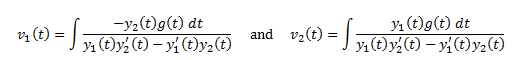
Back to our system of equations for v₁ and v₂: We can solve these equations to obtain

Something to note about these two equations is that the denominators will always be nonzero since they are both the Wronskian. Double hooray!

When we integrate these equations, we get

Now we’ll have a particular solution once we plug these back into y_p = v₁y₁ + v₂y₂.

And now you have a method to solve inhomogeneous differential equations of higher orders! Of course, this method requires for you to first find a fundamental set of solutions to the homogeneous equations, and also to be able to compute those scary-looking integrals for v₁ and v₂, but this method is still important.

That’s it for 4.6! I’ll see you in 4.7!

4.5; the surprisingly short yet very important section.

Section 4.5 is entitled “Inhomogeneous Equations; the Method of Undetermined Coefficients.”

An inhomogeneous equation is of the form y” + py’ + qy = f, where p, q, and f are functions of the independent variable (this variable is usually t). Recall that in the last section (or the section before that, or something) that f is the inhomogeneous term, and we called it the forcing term.

Here’s a theorem for you:

“Suppose that y_p is a particular solution to the inhomogeneous equation [above], and that y₁ and y₂ form a fundamental set of solutions to the associated homogeneous equation

Then the general solution to the inhomogeneous equation [above] is given by

where C₁ and C₂ are arbitrary constants” (164).

We can rewrite this general solution as y = y_p + y_h, where y_h is the general solution to the associated homogeneous equation, i.e. C₁y₁ + C₂y₂.

The method we’ll be looking at this section is called “the method of undetermined coefficients.” We’ll be looking at the inhomogeneous equation y” + py’ + qy = f, where p/q are constants and f = f(t) is a function in terms of the independent variable (in this case, t). It’s important to note that this method works only if the coefficients are constants. The key idea is that “if the forcing term f has a form that is replicated under differentiation, then look for a solution with the same general form as the forcing term” (165). The easiest example is an exponential of the form f(t) = e^at. Then the first derivative f’(t) is also an exponential. There would also be trigonometric forcing terms as well. Here are some examples:

 

Click on it to make it larger. Hooray internet! :D
EDIT: JK, you can't make it larger. Sorry 'bout that.

Something interesting to note when the forcing term is trigonometric is that there is a complex method of solving for particular solutions. If you don’t understand the complex method, this probably won’t be the fastest way for you to solve for stuff. Here’s a website, nonetheless, and following this will be an example: http://tutorial.math.lamar.edu/Classes/DE/ComplexRoots.aspx

 

If the forcing term is a polynomial, we just use this method of undetermined coefficients and solve for our coefficients. Hooray!

Sometimes you’ll get some exceptional cases, like if you get 0 if you insert your solution of a particular form (say, an exponential solution) of the form ae^-t. If this happens, “we look for a solution of the form y(t) = ate^-t. We multiply the usual general form by t. This is the way to find a solution whenever the usual form does not work. If this method does not work, multiply by t once more and try again” (169).

A theorem for you:

“Suppose that y_f(t) is a solution to the linear equation

and y_g(t) is a solution to

Then y(t) = αy_f(t) + βy_g(t) is a solution to…” (170).

Finally, I have a picture summarizing some of the stuff we saw during this section. We can always have more complicated forcing terms, thus paving a narrower path into the realm of “all work, no sleep.” Ah, that blasted place. How I loathe that blasted place.

In any event, I’ll probably see you in 4.6. 

As seen from the 172nd page.

4.4; let's talk physics! (er, harmonic motion)

Section 4.4 is entitled “Harmonic Motion.”

I don’t think you can possibly understand how exciting this is. We recently talked about this stuff in my electronics class. At least, we talked about damping (which this is a very watered down version of it). Hooray physics! :D

The motion for a vibrating spring has the following equation:

In other physics news, in our bonus section from Chapter 3 (the one about electrical circuits), we had the following equation for RLC circuits:

When you compare these two equations, they’re very similar. If we compare coefficients, the inductance L acts as the mass, the resistance R acts as the damping constant, and 1/C (where C is the capacitance) acts as the spring constant. Also, the derivative of the source voltage (NOT energy, which is what I originally interpreted it as) acts as the external force F(t).

Let’s divide our two equations by their leading coefficients (L or m). Then they become

If we change some variables, i.e.

That final equation is known as the equation for harmonic motion. Examples of this equation would be the vibrating spring and RLC circuit. Hooray!

The constant c is called the damping constant, and f is called the forcing term. Finally, this section consists of unforced harmonic motion, meaning that f(t) = 0. This would make our harmonic motion equation homogeneous.

The equation for simple harmonic motion is when there is no damping (i.e. c = 0). The equation then simplifies to be

In the previous section, we know that for characteristic equations with two complex conjugate roots, the general solution will be

In this context, ω₀ is called the natural frequency of the spring. Also, the period of the solution x(t) is denoted as T, where T is defined as 2π/ω₀.

Now, let’s talk a bit about polar coordinates.

Suppose we have a vector (a, b) in the plane. When you write this is polar coordinates and when you assume (a, b) ≠ (0, 0), then there will be a positive number A (which is the length of the vector) and an angle φ in the interval (-π, π] called the polar angle, in which

When you substitute these equations into our general solution, we see we can write the general solution as

In this context, A is the amplitude of the oscillation, and φ is the phase of the oscillation.

Your next question might concern how we find A and φ.

Since we originally defined φ to be any angle between –π and π, then we can’t just take the arctan of b/a, considering that arctan only takes values between –π/2 to π/2. More importantly, this range corresponds to points (a, b) where a > 0. So how do we compute φ when a < 0?

Now let’s consider the case when our harmonic motion is damped (i.e. when c > 0). We’ll have the following differential equation, characteristic equation, and roots:

Now we have a discriminant to worry about, which means we have three cases to consider:

1. c < ω₀; this called the underdamped case. The roots are distinct and complex. The solution would be

2. c > ω₀; this is called the overdamped case. The roots are distinct and real. Also, λ₁ and λ₂ are both positive. The general solution is

3. c = ω₀; this is called the critically damped case. In this case, the root is a double root, i.e. λ = -c. Our general solution is

Here are some websites for you: http://en.wikipedia.org/wiki/Simple_harmonic_motion and http://scipp.ucsc.edu/~haber/ph5B/sho09.pdf and http://wiki.ubc.ca/Simple_and_Damped_Harmonic_Motion and http://hyperphysics.phy-astr.gsu.edu/hbase/oscda.html.

That’s it for 4.4! I’ve been busy and lazy, and that combination leads to me not getting ahead with this blog. We just started chapter 9 in my class, so it’s not like we’re catching up in any way (knock on wood!). Hopefully I can get a lot of chapter 4 up this weekend. If not, maybe I can get one more section up.

I’ll see you in 4.5!

4.3, or the definitely (for real) beginning of our journey through chapter 4.

Section 4.3 is entitled “Linear, Homogeneous Equations with Constants Coefficients.”

These are equations of the form y” + py’ + qy = 0. In this case, p and q are constants. First, we’re going to look at the first-order equation y’ + py = 0. This is an exponential equation, in which its general solution is y(t) = Ce^-pt. In this case, C is just a constant. We’re going to look for a solution of the type y(t) = e^λt, where λ is a constant. When you put this type of solution into the original differential equation,

So Word apparently doesn't like λt...

That final equation is called the characteristic equation for our original second-order differential equation. The polynomial is called the characteristic polynomial, and the roots of this equation are called characteristic roots. Then if λ is a characteristic root, then y = e^λt is a solution to the differential equation.

If you write both the differential equation and the characteristic equation together, then

They look very similar.

The roots for the characteristic polynomial are given by the quadratic formula:

When you look at the discriminant (p² – 4q), there are three cases to consider:

1. Two real roots (p² – 4q > 0)

2. Two complex roots (p² – 4q < 0)

3. One repeated real root if p² – 4q = 0

For the three cases (and the summary), I have a lot of quotes for you. I was doing so well without direct quotes! Oh well…such is life, I suppose.

For two real roots: “If the characteristic equation λ² + pλ + q = 0 has two distinct real roots λ₁ and λ₂, then the general solution to y” + py’ + qy = 0 is

where C₁ + C₂ are arbitrary constants” (151).

For the complex roots, whenever there’s a variable with strikethrough (like this) and it’s also surrounded by brackets, I changed it from an overstrike (which I can’t show in the regular words because overstrikes are hard) to a strikethrough. I thought I’d let you know before you started to wonder why I have brackets around strikethrough stuff.

For two complex roots: “Suppose the characteristic equation λ² + pλ + q = 0 has two complex conjugate roots, λ = a + ib and [λ] = a – ib.

1. The functions

form a complex-valued fundamental set of solutions, so the general solution is

where C₁ and C₂ are arbitrary constants.

2. The functions

form a real-valued fundamental set of solutions, so the general solution is

where A₁ and A₂ are constants” (153). 

For our third case, with the repeated roots: “If the characteristic equation λ² + pλ + q = 0 has only one double root λ₁, then the general solution to y” + py’ + qy = 0 is

where C₁ and C₂ are arbitrary constants” (155).

And finally, the summary of all of this (put in bold and italics because summaries):

“If p² – 4q > 0, the characteristic equation has two distinct, real roots λ₁ and λ₂. A fundamental set of solutions is

If p² – 4q = 0, the characteristic equation has one repeated real root λ. A fundamental set of solutions is

If p² – 4q < 0, the characteristic equation has two complex conjugate roots a ± ib. A fundamental set of solutions is…” (156).

And that’s it for 4.3! I seriously can’t believe I got this done tonight. I’m super excited about this. I don’t have to do this section tomorrow! Hooray!

Enjoy all of the quotes. Also enjoy the beginnings of our journey through Chapter 4.

I shall see you in 4.4! :D

9.9, or the end of a very long, very fulfilling chapter.

Section 9.9 is entitled “Inhomogeneous Linear Systems.”

Inhomogeneous systems have the form y’ = A(t)y + f(t). As before, A is an n × n matrix, y is a column vector for our unknown functions, and f is a column vector of known functions. Recall that it is the f that makes this system inhomogeneous (it’s sometimes called the forcing term).

There’s a theorem, but I’m not going to directly quote it because I know exactly how to say it: The general solution to the inhomogeneous linear system is of the form y = y_p + y_h, where y_p is your particular solution and y_h is the homogeneous solution y’ = A(t)y. In other words, the general solution of the inhomogeneous system is y = y_p + C₁y₁ + C₂y₂ + … + C_ny_n. As they always are, the C’s are arbitrary constants.

If we have a fundamental set of solutions y₁, y₂,…, and y_n to the homogeneous system y’ = Ay, then we could form an n × n matrix Y that contains all these solutions. Thus

This matrix is called a fundamental matrix because its columns form the fundamental set of solutions for the system y’ = Ay.

Here’s a proposition concerning this new information: “A matrix-valued function Y(t) is a fundamental matrix for the system y’ = Ay if and only if…” (445)

An example of a fundamental matrix for y’ = Ay is the exponential e^tA.

Do you remember the variation of parameters thing we did back in the day of single equations? (If not here’s a recap for you: http://differentialequationsjourney.blogspot.com/2013/09/super-serious-and-not-so-funny-linear.html.) For this, we’ll be looking for a solution of the form y_p(t) = Y(t)v(t). In this case, v(t) is a column vector of functions yet to be determined, and Y(t) is the fundamental matrix. I’m going to just state the theorem and skip the derivation, but if you want to know exactly where this came from, I’d suggest looking http://www.mth.msu.edu/~sen/math_235/lectures/lec_20.pdf or http://www.ams.sunysb.edu/~jiao/teaching/ams501_fall11/notes/nonhomo_systems.pdf. They use different variables and they have a few things stated differently than the textbook I have, but it’ll get the job done.

Anyway, the theorem: “Suppose that A is a real n × n matrix and that Y(t) is a fundamental matrix for the system y’ = Ay. Let f(t) be a vector-valued function. Then the solution to the initial value problem

is given by [the following equation]” (447).

The next section is concerning undetermined coefficients. The funny thing about this section is that it references Chapter 4 (which we technically haven’t covered yet) and then gives an example. It has no directions, no outline, or any sort of explanation. After researching on the internet, I have found that this method is used primarily for second-order differential equations (which I thought was to be the case, considering that Chapter 4 details second-order differential equations, which we know because of one of our many bonus sections). I’ll leave a webpage here for the explanation but until we cover it (which we will) I’m thinking we might be glossing over it for now: http://en.wikipedia.org/wiki/Method_of_undetermined_coefficients#Description_of_the_method

One final thing to leave you with for this fine chapter: computing the exponential. Originally, we used the exponential to find the fundamental set of solutions. Now we’re using the fundamental set of solutions to find the exponential of the matrix (funny how things work out, isn’t it?).

The proposition for this is as follows: “Suppose that Y is a fundamental matrix for the system y’ = Ay. Then the exponential e^tA can be computed as

where Y₀ = Y(0)” (450).

Here are some other websites that may or may not help you in the subject of inhomogeneous systems: http://tutorial.math.lamar.edu/Classes/DE/NonhomogeneousSystems.aspx and http://people.math.gatech.edu/~xchen/teach/ode/NonhomoSys.pdf

Other than that, here’s the end of chapter 9. A bit bittersweet, don’t you think?

I don’t. Two more chapters! Twelve more sections! Yay differential equations! :D

I’ll meet you in chapter 4 (again).