9.5: eigens in higher dimensions! :D

Section 9.5 is entitled “Higher-Dimensional Systems.”

Let us start out with a proposition and a theorem.

The proposition: 

“Suppose λ₁, … , λ_k are distinct eigenvalues for an n × n matrix A, and suppose that v_i ≠ 0 is an eigenvector associated to λ_i for 1 ≤ i ≤ k.

1. The vectors v₁, … , and v_k are linearly independent.

2. The functions

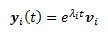
1 ≤ i ≤ k, are linearly independent solutions for the systems y’ = Ay” (408).

And the theorem:

“Suppose the n × n matrix A has n distinct eigenvalues λ₁, … , and λ_n. Suppose that for a ≤ i ≤ n, v_i is an eigenvector associated with λ_i. Then the n exponential solutions

form a fundamental set of solutions for the system y’ = Ay” (408).

This theorem is most useful when eigenvalues of a system are real. This means the exponential solutions will also be real. This means the general solution will be of the form

As usual, C₁ through C_n are arbitrary constants.

(Allow me to stop right here and point out that the word “arbitrary” has been used so many times in this book. It must be the authors’ favorite word (or a favorite in the study of mathematics)).

This theorem also applies when eigenvalues (some or all) are complex; the only condition is that the eigenvalues must be distinct.

More generally speaking, if we have two eigenvalues λ and λ, which are what the book calls a “complex conjugate pair.” As we learned earlier in the chapter, these two eigenvalues have associated eigenvectors w and w. These pairs form complex conjugate solutions

The real and imaginary parts of z are solutions. Also, if z and z are linearly independent, then the real and imaginary parts x = Re(z) and y = Im(z) are also linearly independent.

So the general method of finding a set of solutions for a system x’ = Ax is to find the eigenvalues, either by hand or with a calculator/computer. If the eigenvalue is real, then we can use the method in the theorem from section 9.1. We use the equation

From this equation, we can find our eigenvectors. But say we want to find the eigenvectors for complex eigenvectors. The book says to use a computer/calculator. Then you can use Euler’s formula (en.wikipedia.org/wiki/Euler's_formula) to find the real and imaginary parts of the associated solutions with the complex eigenvalues and eigenvectors. You’ll have a real and imaginary part of this solution, but we know that both parts are solutions.

So we talked about how the eigenvalues should be distinct, but there are some cases where eigenvalues are repeated. If you’re wondering how that works, suppose we have a matrix where the characteristic polynomial is p(λ) = λ³ + 5λ² + 8λ + 4, which would factor to be (λ + 1)(λ + 2)². Thus our eigenvalues would be -1, -2, and -2. We would kind of expect repeated eigenvalues would make everything a living nightmare, but sometimes that doesn’t happen. Sometimes repeated eigenvalues need what the book calls “special handling,” but allow me to remind you that this is a textbook and thus the examples are not usually pulled out a thin air. We’ll find ways to solve for repeated eigenvalues.

Apparently, in the next section, we will find a way to solve for solutions where there are repeated eigenvalues, so I guess we’ll cross that bridge when we come to it. For now I will leave you with this: http://www.sosmath.com/diffeq/system/linear/eigenvalue/repeated/repeated.html

If A is an n × n matrix with real entries, then we’ll have a list of eigenvalues λ₁, λ₂, …, λ_k, that are distinct. (So if we went back to our characteristic polynomial above, our list of distinct eigenvalues would be -1 and -2.) In general terms, the characteristic polynomial of A will factor into

The powers must be at least 1 and the sum of the powers will equal n (i.e. q₁ + q₂ + … + q_k = n). So in our example of a characteristic polynomial, our q₁ = 1 and q₂ = 2 because those are the powers when we factored our characteristic polynomial. The algebraic multiplicity of λ_i is q_i. The geometric multiplicity of λ_j is d_j, where d is the dimension of the eigenspace of λ_j.

If d_j = q_j for all j, then

This would equal the total of solutions. In this case, we would have a fundamental set of solutions. The beautiful thing about this is that we don’t really need distinct eigenvalues; we can find a fundamental set of solutions provided that the each eigenvalue’s geometric multiplicity is equal to its algebraic multiplicity.

If they aren’t equal…well, we’ll deal with that in the next section. I’ll see you in 9.6!