8.2: A lot of words about pretty pictures of graphs

Section 8.2 is entitled “Geometric Representation of Solutions.”

The model we’re going to use this section is called the Lotka-Volterra model of predator-prey populations. I’m not going to derive it; rather, I’ll hand you the final system and you can take my word that it’s all correct:

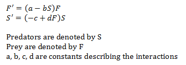
This model is nonlinear and autonomous.

One way you can represent this model is to plot all of the components of the solution. You can probably Google it (or go here http://en.wikipedia.org/wiki/Lotka%E2%80%93Volterra_equation or here http://mathworld.wolfram.com/Lotka-VolterraEquations.html) but the graphs seem to be a periodic variation of the populations of predators and prey.

Another way we can see the solution is to look at a parametric plot. Let’s set u(t) = (F(t), S(t))^T and plot t → u(t) = (F(t), S(t))^T. This view would be in R², so we can call this solution curve a phase plane.

To see the phase plane of the Lotka-Volterra model, you can go here: http://mathinsight.org/applet/lotka_volterra_phase_plane_versus_time_population_display

For those of you who are too lazy to click on the link (or copy-paste), it looks like an egg. More specifically, it shows how the two populations interact. A fancy term for “egg” is “closed curve”, which means it tracks over itself as time increases. This makes sense, if we are to believe that the solution is indeed periodic. The derivative u’(t) is a vector tangent to our egg at a point u₀ = u(t₀).

This kind of analysis can be done for higher dimensions, (t → y(t) is the parameterization for a curve in Rⁿ, and y’(t) is a vector tangent to the curve at y(t)). It’s just much harder to visualize once you go into dimensions higher than 3.

Now let’s suppose we have a planar system:

In this case, y(t) = (y₁(t), y₂(t))^T would be a solution. We could look at the solution curve t → y(t) in the plane. In this case, this y₁y₂ plane is still called the phase plane, but solution curve is called the phase plane plot or solution curve in the phase plane.

Generally, we’ll be in dimension n and our equation will have the form x’ = f(t, x). The x-coordinates would be called the phase space, and the plot of the curve t → x(t) is called the phase space plot. They’re pretty important for autonomous systems.

Let’s consider the autonomous system

Note this is autonomous because the independent variable doesn’t appear explicitly on the right-hand side. Let’s assume that f and g are defined in a rectangle R in the xy-plane. Let’s consider the solution of the form (x(t), y(t)) and the curve t → (x(t), y(t)) in the xy-plane. This means there will be a vector

that will be tangent to this curve. So if we assign a vector to each point in our rectangle R, then we would have what is called a vector field of our original system. For a pretty picture of the Lotka-Volterra vector field, you can go here http://mathforum.org/mathimages/index.php/Field:Dynamic_Systems#Maps

If we picked a starting point, then the vector field would show us how that curve would form and what our egg would look like. Ultimately, the curve goes back to our original point, which makes sense since we have an egg and not a bowl (or some equivalent open-ended egg shape).

Now let’s start with the general system

Now f and g are defined in a three dimensional shoebox R. This would be in the (t, x, y) space. The limits on this space, in a more general form, would be

In this case, the vector field would be (f(t, x, y), g(t, x, y)), which means it now depends on t, x, and y. Well, if t can change as well, then it doesn’t make much sense to observe a vector field in the phase plane. In this case, we will be looking at a three dimensional direction field.

We’re going to consider the curve parameterized by t → (t, x(t), y(t)) in our shoebox R. This time, our tangent vectors will take the form

Something interesting to note about this is that the vector (1, f(t, x, y), g(t, x, y)) can be computed without knowing the solution of the system. This type of interpretation of our system will be called (surprise, surprise) a direction field.

The solution to the Lotka-Volterra model in a three-dimensional direction field looks really awesome. While my skim of the internet didn’t produce a website that could accurately depict this phenomenon, I encourage you all who have a copy of the book to take a look (page 344).

Since we discussed three different ways to visualize solutions, you can put them all together in a composite graph.

There’s no best way to visualize one of these solutions. The book encourages you to look at all of the visualizations. I encourage you to get correct answers and pass tests (and understand how to visualize these things).

Finally, a thing from the book concerning higher dimensions: “What do we do in higher dimensions? What we do not do is become daunted by the seeming impossibility of visualizing in dimensions greater than 3. Instead we try anything that that seems like it will be helpful” (345).

Don’t be daunted, my friends. I’ll see you when I see you.