The end of a chapter, but the beginning of a beautiful understanding of differential equations.

Section 2.9 is entitled “Autonomous Equations and Stability.”

So a first-order autonomous equation has the form x^’ = f(x). This is a neat function because the independent variable doesn’t appear explicitly on the right hand side of the equation. We’ve already seen an example of an autonomous function, and that would be the differential equation the air resistance proportional to the square of the velocity. That equation was the following:

The independent variable t does not appear anywhere on the right hand side of the equation, and thus this equation is autonomous.

These types of equations actually happen often in real world applications. Note: “A differential equation model of any physical system that is evolving without external forces will almost always be autonomous” (92).

Another cool thing about autonomous equations is that the slopes of the direction lines in the direction field have the same feature.

We see that the slopes don't change as you move from left to right. (sosmath.com)

Qualitatively, we can find some really easy solutions pretty quickly. For example, If f(x₀) = 0, then x(t) = x₀ satisfies x^’(t) = 0 = f(x₀) = f(x(t)).

Some definitions for you: the point x₀ which satisfies f(x₀) = 0 is called an equilibrium point. This constant function that arises because of the point x₀, which is x(t) = x₀ is called an equilibrium solution.

So, returning to our air resistance function, we look at the right hand side of the equation and find that

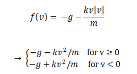
Something important to point out is that f is a decreasing function. This means it can only have one zero. F will be positive when v is greater than zero, so this means that our zero (AKA our equilibrium point and solution) must occur when v is less than zero. We have an equation for that, so when we solve for v, we get that our equilibrium point and solution is

Tying back to what I attempted to summarize/teach you in the last section (2.7, about uniqueness and existence and all that noise), the function f and its derivative “-2k|v|/m” are both continuous for v. This means the uniqueness theorem is satisfied and that’s just fantastic. This also means equilibrium solutions (i.e. solution curves) cannot touch. This means we have

When v(t) satisfies this, then f(v(t)) < 0. This means that

This makes v(t) a monotonic decreasing function (remember those fancy words from Calculus 1?). While we’re on the subject of Calc 1, let’s look at the respective limits of this function. As t goes to infinity, v approaches –sqrt(mg/k), and as t goes to negative infinity, v approaches infinity.

So, for an initial value problem v(t₀) > -sqrt(mg/k) with the solution v(t), we can make three observations:

1. v(t) is monotone decreasing

2. v(t) goes to –sqrt(mg/k) as t goes to infinity

3. v(t) goes to infinity as t goes to negative infinity

Notice for our second observation, notice that we got this answer back in section 2.3; we just called it terminal velocity.

Moving on, our autonomous equation y^’ = f(y) describes the motion along y(t). This makes sense since y^’ is a derivative and it involves slopes and motion and stuff. (Definition alert) a phase line is the line along which y^’ describes motion.

The horizontal line would be the phase line. 

Just a reminder, the point on the v line is our equilibrium point, -sqrt(mg/k). Obviously, the left has our f(v) increasing, so we indicate it with the blue arrow pointing to the right. The right side of the equilibrium point is the opposite; it’s decreasing, and we show that with the arrow pointing to the left.

If you have more than one equilibrium point, you will have more than one phase line.

Let’s talk about stability now.

Sometimes, you have solution curves that approach your equilibrium points as t becomes infinite. The special name for these points is “asymptotically stable equilibrium points.” Sometimes, your solution curves move away from your equilibrium points. These points are deemed unstable equilibrium points. In terms of a graph, if your two arrows that you draw on your graph point toward your point, then it’s an asymptotically stable point.

So you might be saying at this point, “by golly I want to deem points stable and unstable and other [these are called semi-stable, but the book says not to stress about it]. I would like to know how I can determine the stability of my equilibrium points.”

Well, by golly, I have a first derivative test for stability for you!

“Suppose that x₀ is an equilibrium point for the differential equation x^’ = f(x), where f is a differentiable function.

1. If f^’(x_0­) < 0, then f is decreasing at x₀ and x₀ is asymptotically stable.

2. If f^’(x₀) > 0, then f is increasing at x₀ and x₀ is unstable.

3. If f^’(x₀) = 0, no conclusion can be drawn” (98).

Okay, now that we know everything there is to know about autonomous equations (well, we can pretend we know everything), we have a method to solve these pesky little things. I’m going to use a direct quote on this too since, you know, summarizing a summary wouldn’t work out so well.

“1. Graph the right-hand side f(x) and add the phase line information on the x-axis. Find, mark, and classify the equilibrium points where f(x) = 0. In each of the intervals limited by the equilibrium points, find the sign of f and draw an arrow to the right is f is positive and to left if f is negative.

2. Create a tx-plane, transfer the phase line information to the x-axis, draw the equilibrium solutions, and then use the phase line information to sketch non-equilibrium solutions in each interval limited by the equilibrium points” (99).

That’s all for this section, I’m afraid. You’ll hear from me when we move into the magical land of chapter 3. I’ll see you when I see you! :D