3.1: A lot of words about amoebas

Section 3.1 is entitled “Modeling Population Growth.”

Population growth is a beautiful real-world application of differential equations. Because modeling human population growth is too mainstream, we’re going to look at the population growth of single-celled organisms called protozoa. These would be organisms such as amoebas (which is a really fun word to say really slowly).

But first, let’s use some exposition about the life and death of these organisms in order to have underlying context for our differential equation.

Simply put, protozoa use cell division and there’s plenty of room and food to grow and every cell divides the exact same way. In some time interval (in which time is measured in an intelligent manner, like hours or days), there will be about this many divisions:

In this context, b is known as the birth rate (since this is for multiplying cells). The birth rate is simply a probability one of these protozoa will divide within a certain unit of time (which will be whatever we pick, e.g. hours or days).

Now, supposing that protozoa will die eventually, we’re going to use a very similar equation to our multiplication/birth equation. Instead of a birth rate, we’re going to denote d as the death rate, which is just the probability a protozoa will die given a certain unit of time.

Thus our equation will be

 

So now we have two equations relating to the birth and death of these organisms. If we combine them to form one super population model between the times t and t + Δt (where Δt is just our interval of time where we observe life and death of amoebas),

So, when we take the derivative, we get the following:

(Note: the book uses the “limit quotient definition” of the derivative, which is neat. If you don’t know what that is, here’s a handy webpage that has examples and definitions and stuff: https://www.math.ucdavis.edu/~kouba/CalcOneDIRECTORY/defderdirectory/DefDer.html)

The model P^’ = rP is a standard model for the growth of a population. It’s quite common to call r a reproductive rate. It’s also a first-order differential equation involving the function P(t).

Moving on, we originally made the assumption that our organisms have plenty of room and space to grow and be happy. This would make our birth and death rates constant (and thus r would be a constant as well). This would make our differential equation really easy to solve, and we can just use our handy separation of variables technique to bring us to the solution

C can be positive, negative, or zero. Something to notice about this is that at time t = 0, the exponential goes to one and we’re left with an initial population (which would be our C constant). Thus, a better version of our solution would be

This model is called the Malthusian model, named after the guy who came up with it. There are two cases to consider with the Malthusian model. If our death rate is larger than our birth rate, then we get a negative reproductive rate, which means our population will decline. If our birth rate is larger than our death rate, then we get a positive reproductive rate, which means our population will increase.

Just as a recurring example for this section, let’s suppose we’re growing some bacteria for a project or something. Let’s start with 100 individual bacteria at time t = 0, and let’s say our reproductive rate is 0.5. This would make our equation

Simple enough? I sure think so.

For some context (and to show how exponential our function is), if we measure our time in hours, after 24 hours the model suggests we will have approximately 16,275,479 bacteria.

Obviously, our constant r has to reflect the real-world. It’s fairly easy to find r, so let’s just do that now:

Suppose we still start with 100 bacteria, and when we check back in 24 hours and we count 250 bacteria in our sample. We start with our general solution to our differential equation:

At time t = 0, we have 100 bacteria, so this would be our P₀. If we put our time in units of days, then at time t = 1, we have 250 bacteria. Plugging this in,

In a week (time t = 7), our model suggests

That’s nice and all, but if we wanted a better model for our population, we would count our bacteria population every day and create a better model from our refined data. In order to re-estimate our r, we can use a process called linear regression. For the most part, we’re going to use a calculator to do linear regression, but let’s better understand what our calculator is doing to get the job done.

So if we start with our general solution to our differential equation, we take the logarithm of each side, which results in the following:

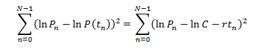
Note that the natural log of P(t) would be considered a linear equation (recall section 2.4) with respect to t with our coefficients being “rt” and the natural log of C. We’re going to make new measurements of our population N times, for t₀, t_1, all the way to t_N-1, and we will get populations corresponding to those times P₀, P₁, all the way to P_N-1. So the actual method of linear regression chooses the natural log of C and r to minimize the function

The method of linear regression is also a case of another method called the method of least squares (which, in my opinion, is a pretty awesome name for a method). This is what your calculator does when you ask it to perform a linear regression when you want to re-estimate your reproductive rate.

Now you know how to make a better estimate for our fake project!

(Note: I was going to show an example of this, but it’s not very fun to write out or perform, so I’m not going to write it out. Suppose we still start out with 100 bacteria and over a four day period we count 250, 615, 1500, and 3800 bacteria. These would respectively correspond to t = 1, 2, 3, and 4, with t = 0 having a population of 100. If you have a calculator that is a TI 83 or 84 plus, here’s a handy website to figure out linear regression: http://www.calcblog.com/performing-a-linear-regression-on-the-ti-83-or-ti-84/)

Moving on, let’s think a little more deeply about our Malthusian model for population growth. Obviously, the model is impossible since it’s an exponential function that is basically unlimited in its growth. In a real world context, if amoebas grew exactly how the Malthusian model predicts, then our world would be covered in amoebas and that’s not a thing that occurs IRL. This is obviously a major character flaw in our model.

But we did inflict this character flaw upon ourselves when we assumed that our single-celled friends have no restrictions on food or space. This is the real world, where we can’t feed every amoeba or provide a home to every amoeba family. Although these assumptions are perfectly fine the cases for smaller populations (and our exponential growth function has been verified for small populations in real-world labs), we need to consider the limits of growth for larger populations.

In order to consider the limits of growth, let’s look a little more closely at our death rate. A lack of food for every living amoeba means that some will starve or die from malnutrition (I know, the world is brutal). This means there will be a competition among amoebas to get food, which increases the interaction among amoebas. A lack of space means amoeba families will compete for space, and there will be more deaths due to this increased interaction. Long story short, the death rate will increase due to the increased interaction. This means the death rate increases proportionally to population size. This would make our new formula for our death rate: “d + aP.” The d is still the death rate for small populations (i.e. the death rate we found before). The thing we have changed to account for larger populations is the “aP” term, which will measure the new deaths due to increased interaction. The constant a will measure the actual impact these interactions will have on the death rate.

At the same time, our birth rate will change as well. We will have the new formula “b – cP,” where the b is the same as before.

So, recall at the beginning of this chapter we looked at the change of population between t and Δt, and then we took the limit quotient definition of the derivative. We will get the following result:

To make this answer look a little nicer, let us denote the quantity “b - d” r₀. Instead of calling this the reproductive rate, we will call r₀ the natural reproductive rate. Let us also denote the quantity “a + c” as r₀/K, where K is just some new constant we just made up. This means our equation will look like this:

This equation is called the logistic equation. This model for population growth is called the logistic model (which is not named after the person who postulated it). If we think about r in terms of the equation P^’ = rP, then we see that

This means that r is no longer a constant. This also means that r will be negative if P is larger than K.

Recall in section 2.9 what an autonomous equation is, and notice that our logistic equation is an autonomous equation. This is because the right-hand side of that function does not depend on time (which t is our independent variable). This means we can make one of those handy graphs with those neat blue arrows that tell us our equilibrium points.

Well, we don’t even need the graph to tell us our equilibrium points. Recall that equilibrium points are wherever f(P) = 0. This would be when P = 0 and when P = K.

As you can see by the graph, P = 0 is considered an unstable equilibrium point and P = K is a stable point. What does this mean? Note: “…if P(t) is any solution with a positive population, then it must stay positive, and it must tend to K as t → ∞” (109). This means that every positive population that is modeled by the logistic equation will tend to K as time increases. This is why K is known as the carrying capacity.

Now, you might be saying, “Erin, hold up. Aren’t all populations positive?”

To which I answer, “Well yes, but this is math, where population models can have negative solutions.”

To which you say, “Okay, fine. Well, how do we solve these logistic equations?”

To which I stop talking to you and just use math words and numbers now.  

The book now drops the 0 in our r₀ and our equation becomes

Since our equation is autonomous, it is also separable. Thus we rewrite this equation as

And now we integrate. Notice we must use partial fractions to integrate the left hand side. If you don’t remember what partial fractions are, here’s a handy website for you: http://tutorial.math.lamar.edu/Classes/CalcII/PartialFractions.aspx

After integrating, we arrive at the following equation:

If we replace the e^C with the constant A that can be positive, negative or zero, then we can drop the absolute value signs and therefore write our equation as

We already stated that as time becomes infinitely large, then our function will go to K. If you take the limit of our newfound equation, you will see this is the case.

Given three observations or estimates, then we will be able to find our constants (P₀, r, and K). If the times of these measurements are equally spaced (say t₀ = 0, t = h, and t = 2h), and at those times we measure populations of P₀, P₁, and P₂, then if we solve our equation for K, we get

From here, we can substitute this value of r into one of our two equations for K and solve.

Finally, in the book there is an example that deals with real-world data. Because the real world is real life and therefore full of human and experimental error, we can find error in our K value, and curve of best fit to real-world data. This example also uses the method of least squares to minimize error. The result of this is called a least squares approximation. However, this is different than what we had learned before because this example deals with a nonlinear least squares problem. If you care at all about nonlinear least squares, then here’s the Wikipedia page for it: http://en.wikipedia.org/wiki/Non-linear_least_squares

This is all I have for you this section. I’ll see you when I see you.