2.6 - SO MANY WORDS AND NUMBERS

Section 2.6 is entitled “Exact Differential Equations.”

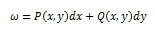
Let’s look at a very general differential equation

You work this differential equation like you would work any other differential equation; you can solve for y(x) and our differential equation will satisfy it. Recall that back in our discussion with separable differential equations, we talked about solutions that are defined implicitly. This means they take the form

In this equation, x and y are treated the same. There is no distinction between the two. We can do this for any differential equation. This leads us to a definition:

A differential form for x and y has an expression like

P and Q are still functions of x and y, like our first equation. The dx and dy in the expression are called differentials. Y is still the dependent variable, so it can still be written as y(x). This means

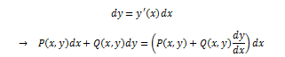
Y is a solution to our original differential equation if and only if

This is just another way of writing our original differential equation.

Now, let’s suppose that the solutions for our differential equation (we can refer to either form for this) are given implicitly by F(x, y) = C. The level sets defined by our solutions are called integral curves.

(Wikipedia)

The picture shows integral curves for differential equation

Also, here’s a website that draws solution curves for pretty much any equation you want: http://faculty.fortlewis.edu/Pearson_P/jsxgraph/slopefield.html

Moving on, we said F(x, y) = C gives a general solution for the following equation:

So y = y(x) is defined by our general solution. When we take partial derivatives in terms of x, we get

If you don’t remember what a partial derivative is or how to take a partial derivative, I’ll leave this handy website for you here: http://tutorial.math.lamar.edu/Classes/CalcIII/PartialDerivatives.aspx

We already said y(x) is a solution to our differential equation, so we graciously receive

When we compare our two previous equations, we see that

If we define the latter part of our previous equation as μ(x, y), then our equation simplifies to be

Therefore, in order to find a solution to our original differential equation, we must find the functions μ and F that satisfy our previous equations.

Right now, we’re going to look at when μ = 1, which would make our equation:

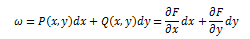
Note: “The differential of a continuously differentiable function F is the differential form

A differential form 

is said to be exact if it is the differential of a continuously differentiable function” (65).

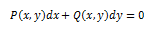
In other words, the form “P dx + Q dy” is exact if and only if there’s a function F(x, y) such that

This means dx = dy, or

Also, if the form “ω = P dx + Q dy” is exact and equal to dF, then the general solution to “dF = P dx + Q dy = 0” is given by F(x, y) = C.

Here’s an example (and there are two others on Khan Academy so you could watch all of them if you’d like): https://www.khanacademy.org/math/differential-equations/first-order-differential-equations/exact-equations/v/exact-equations-example-1

It’s fairly easy to solve a differential equation when its variables are separated. In terms of our original differential equation, that form would be P(x)dx + Q(y)dy = 0. The solution to this would be F(x, y) = C, where

From this, two questions can arise:

1.     When ω = P dx + Q dy, how do we know if it’s exact?

2.   If it is indeed exact, how do we find F such that dF = P dx + Q dy?

To answer these questions, let us use the equation from our first question, where P and Q are continuously differentiable. Here’s a two part theorem about this equation:

(a)  If ω is exact, then

(b)  If this equation is true in a rectangle R, then ω exact in that rectangle.

The proof is done by hand for you (you’re welcome, although it wasn’t that hard):

So to solve an exact differential equation, we have two methods to do so:

1.  Find F by guess-and-check (but the book is for grownups and the grownup version of this is “inspection and experimentation”)

2. Use the second part of our proof.  Reminder: If “P(x, y) dx + Q(x, y) dy = 0” is exact, the solution is F(x, y) = C, where F is found by solving

Here are some steps to follow:

You could solve in terms of Q (it would be with respect to y instead of x) first, but there would be a different “constant” of integration (instead of phi).

Moving on:

Let’s flashback to where we said in order to solve “P dx + Q dy = 0” we need to find a μ and F that satisfy

Here’s a new definition: “An integrating factor for the differential equation “ω=P dx + Q dy = 0” is a function μ(x, y) such that the form “μ ω = μ(x, y) P(x, y) dx + μ(x, y) Q(x, y) dy” is exact” (69).

In order to find a general solution to P dx + Q dy = 0,

1. Find an integrating factor μ  so that “μ P dx + μ Q dy” is exact

2.  Find a function F such that “dF = μ F dx + μ Q dy”

Our general solution takes the form F(x, y) = C.

So in this context, let’s redefine separable and linear equations.

An equation is separable if there is an integrating factor that separates the variables in the form P(x) dx + Q(y) dy = 0. This means the solution is given by

Back in section 2.2, there was a special case in the form

So the integrating factor would be q(y), and the equation transforms to “p(x) dx – q(y) dy = 0”

Linear equations have a special form

Back in section 2.4, we solved a linear equation using an integrating factor μ(x)

If μ(x) satisfies this equation, then “μ(x)[a(x) y + f(x)]dx - μ(x)dy = 0” is exact. This means the general solution is

Moving on, suppose ω = P dx + Q dy and we want a μ such that “μ ω = μ P dx + μ Q dy” is exact. This means μ must satisfy

However, there really is no procedure for solving this equation. It would make it easier to have an integrating factor that only depends on one variable, because then this equation would be so much easier to solve. Let’s just do that for now.

So let’s find out when P(x, y)dx + Q(x, y)dy = 0 has a μ(x) that only depends on x. This means μ does not depend on y (common sense) so our equation would simplify to be

So μ will only depend on x solely if the following equation solely depends on x:

If this is true, then μ(x) is a solution to

More generally, “P dx + Q dy” will have an integrating factor that only depends on one variable under these conditions:

Moving on, here’s a handy definition of a homogeneous equation: A function G(x, y) is homogeneous of degree n if G(tx, ty) = tⁿ G(x, y) for all t > 0 and x ≠ 0, y ≠ 0

Here are some examples of homogeneous functions:

Their homogeneous degrees are -2, 0, 3, and 1, respectively.

Here are some examples of non-homogeneous functions:

“P dx + Q dy = 0” is homogeneous if P and Q are homogeneous to the same degree. We could also put these equations into a solvable form using the substitution y = xv (where v is a new variable). Here are some steps to make this easier:

1. Make the substitution y = xv

2.  Look for an integrating factor to separate the variables.

Let’s start with P(x, y)dx + Q(x, y)dy = 0, where P and Q are both homogeneous to the same degree.

If y = xv, then P(x, xv)dx + Q(x, xv)(v dx + x dv) = 0

We stated above that P and Q are homogeneous. This means 

P(x, xv) = xⁿ P(1, v) and Q(x, xv) = xⁿ Q(1, v)

When we use this, our differential equation becomes

[P(1, v) + v Q(1, v)]dx + x Q(1, v) dv = 0

Our integrating factor would be

This will separate our variables, so it leaves us with

Then we can substitute v = y/x back into our function so we can have our y’s back in the equation.

Finally, here are some examples from the book that may or may not help you understand this better.