7.2, moar dimensions = moar fun

Section 7.2 is entitled “Systems of Linear Equations with Two or Three Variables.”

Let’s consider the equation 5x + 7y = 9. There will be a lot of different vectors that will satisfy this equation (i.e. solve it). The set of all of these vectors will be known as the solution set. In this case, the solution set would be a line in the xy-plane.

If we solve for y, we’ll get y = (9 – 5x)/7. This can be rewritten as

This equation is known as the parametric representation of the line modeled by our original equation. In this case, x is a free parameter, because any value of x will be a point on the line. For example, when x = 1, a point (1, 4/7)^T would be on the line. 

Generally, we would start at x = 0, and then that point would be called p. Then, for any value of x, we would add multiples of the vector v = (1, -5/7)^T.

(Reminder: The T is a transpose, and it’s just being used as a handy way to write vectors horizontally, despite their vertical traits.)

Time for our favorite words again!

Ax = b is said to be homogeneous if b is equal to the zero vector, which the book denotes by 0. If b is not equal to the zero vector, then the system is inhomogeneous.

And now for a definition:

“A line is Rⁿ is a set of the form

where p and v ≠ 0 are vectors in Rⁿ. [This equation above] is called a parametric equation for the line” (284).

The vector p is the point corresponding to t = 0. Our vector v gives us the direction of the line.

Now let’s look at two linear equations with two unknowns. Let’s consider the following equations:

5x + 7y = 9

x – y = 0

Separately, the solution sets for these equations are lines. Since we want the solution for both equations at the same time, then we’re looking for the line in which these equations intersect. Either there will be one point they intersect, or they will never intersect (because then they would be parallel).

We could solve this equation using algebra, by substituting x = y into our first equation and then getting answers. We would get 12y = 9, which would lead us to the new system of equations x – y = 0 and 12y = 9. We could add 12 times the first equation to the second and solve for x. This operation is called elimination (because our goal is to eliminate variables). Or you could just solve for y in our second equation and plug into the first equation to solve for x. Either way, you get the answer to be x = y = 9/12 = 3/4.

If we solved the second (i.e. last) equation first in our new system of equations and then solve the first equation, then we would be performing the method of back-solving. However, we usually have too difficult of equations and unknowns to simply back-solve and be on our merry way. We will usually use elimination to solve our equations.

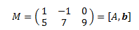
Let’s rewrite our system in matrix notation:

If we define A as our coefficient matrix and b as the right hand side, we can rewrite this system as A(x y)^T = b. All of our information can be easily compacted into one larger matrix, called the augmented matrix.

We could also solve this matrix to look like our second set of equations, i.e. adding -5 times the first row to the second row. Then we would get

If the equations in a system are parallel, then they will have no solution. We call these systems inconsistent. We could also be presented with a system with equations that are multiples of each other. In this case, their solution sets would be the exact same. In conclusion of this, there are three and only three outcomes for solving a system of equations:

1. One point

2. A line

3. No solutions

Our first case happens often. The other two cases are called degenerate cases.

A bit more on homogeneous systems: They will always be consistent. So if you are presented with a homogeneous system, then you will never get “no solution” as the answer. The solution will either be the origin, or the line going through the origin.

If we were offered the line x + 2y – 4z = 5, then that equation is in three dimensions. We could solve this equation for x and get x = 5 – 2y + 4z. Then we would have the solution set be

Similar to the equation in two dimensions, this would be the parametric representation for a plane. In this representation, we have two free parameters: y and z. We would start at our point p = (5 0 0)^T and adding a linear combination of what is called v₁ and v₂. 

The formal definition:

“A plane in Rⁿ is a set of the form

where p, v₁, and v₂ are vectors in Rⁿ such that v₁ and v₂ are not multiples of each other. [The equation above] is called a parametric equation for the plane” (287).

If we were to look at two equations with three unknowns (which will make planes), then we know by geometry the solutions will have three possibilities:

1. The planes intersect in a line

2. The planes are the same plane and thus the solution set will be a plane

3. The planes are parallel and there will be no solution

In order to solve these equations, we shall use matrix notation and elimination. In some cases, we can eliminate some things and then make it possible to back solve. Then, in that case, we may be able to assign any value to a certain variable, say z, and then we can easily solve for numerical values for the other two variables, say x and y. In this case, we would call z a free variable and then we can set z = t (it’s the book way of saying, “hey, this can be any number”). This means the solution sets for planes will take on the following form:

This is just an example, but shows what our solution sets would look like.

For three equations and three unknowns, we will use matrix notation and elimination to prepare for back-solving. It sounds fairly simple, but it really can get messy. If you pick the right numbers, the answer can look gross. The solution sets for three equations with three unknowns will either be

1. One point

2. A line

3. A plane

4. No solution

If the equation is homogeneous, then the origin will always be a solution, which means homogeneous solutions will always have a solution. This means our possibilities for homogeneous systems are

1. The origin

2. A line though the origin

3.  A plane through the origin

Notice that we can have a single point as a solution for one, two, or three dimensions. This will look similar in any dimension. We also have lines in two dimension and lines and planes in three dimensions. They have common features that the book describes well:

“First, if we can move in a particular direction…we can move arbitrarily far in that direction. We can summarize this by saying that the set in infinitely long. Second, if there are two are two directions in which we can move, as in a plane, then we can move in any linear combination of those directions. We can summarize by saying that the solution set is flat. Finally, a line in the plane, or a line or plane in 3-space, does not take up much room. Both have negligible extent in most directions. We can summarize that by saying that the solution set is thin” (290).  

When we go into higher dimensions, we can’t really visualize it anymore and our intuition is lost. But we might think that these characteristic (long, flat, and thin) might also be used to describe solution sets in higher dimensions.

I guess we’ll find out when we go to section 7.3, but for now this is where we will end.

I’ll see you when I see you!