Section 7.3 (row reduced madness)

Section 7.3 is entitled “Solving Systems of Equations.”

I’ll just start with the definitions and then show an example.

“The pivot of a row vector in a matrix is the first nonzero element of that row” (292).

So the first row, first column position (1), the second row, second column position (6), and the third row, fourth column position (16) are pivots.

“A matrix is a row echelon form (or just echelon form) if, in each row, that contains a pivot, the pivot lies to the right of the pivot in the preceding row. Any rows that contain only zeros must be at the bottom of the matrix” (293).

An example of a matrix in row echelon form:

Generally speaking, a matrix in row echelon form looks somewhat like this:

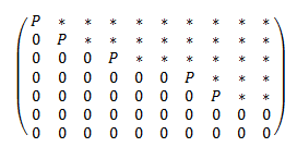
Where P represents some number that is the pivot of that row and the asterisks are arbitrary numbers.

If you want an example (video, steps, etc.): http://www.wikihow.com/Reduce-a-Matrix-to-Row-Echelon-Form

In order to get a matrix (and thus a system of equations) into row echelon form, we have three row operations we can perform:

1. Add a multiple of one row to a different row.

2. Interchange two rows.

3. Multiply a row by a nonzero number.

With these three row operations, you can literally (and I do mean literally) put any matrix into row echelon form.

If a matrix is in row echelon form, then there can be at most one pivot in each column. Then this column would be known as a pivot column, and the variable would be known as a pivot variable. The columns that are not pivot columns would be called a free column, and then the variable in that column would be known as a free variable. This is because you can assign any arbitrary value to this variable.

So then we’re down to a general formula to follow when trying to solve any linear system Ax = b. We first form the augmented matrix M = [A, b], then use row operations to reduce M to row echelon form. Once we have that simplified system, we can solve by assigning values to the free variables and then perform back-solving to find values for pivot variables.

So your next question might be, “How do we know when we don’t have a solution?”

This matrix basically says 0x + 0y = 8, or 0 = 8, and that’s not right. That’s not a thing that can happen in math. This system would be inconsistent and have no solutions.

The important thing to take from this is that a system is consistent if and only if it doesn’t have a pivot in the last column of its augmented row echelon form.

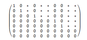
So if it’s possible, you can put your matrix in row reduced echelon form, in which your pivots are ones and the terms above your pivot variables are zeroes.

It’s your choice which form you want to bring your systems to. Row reduced requires a lot more work, but it’s super easy to solve. It’s really up to your tastes on what kind of work you want to do.

As a testimonial to you, the way this really makes sense is to work on examples, do the row operations, and watch the shapes form and the numbers work. You can find a hundred examples of matrices you can row reduce (or you can make your own, but they might become super gross super fast) and when you start to work on them, you’ll get better at noticing the patterns and understanding what needs to happen to make your life easier.

All right. I’ll see you in 7.4.