Section 7.6 is entitled “Square Matrices.”
Square matrix has the same number of rows as columns
(surprise, surprise!). This also is equivalent to a system of n equations with
n unknowns. There are really interesting and lovely conclusions we can conclude
about matrices that are square, and that’s basically what this section is all
about.
Note: whenever I speak of the matrix A, A will always be a
square matrix. In other words, A will be an n × n matrix. I’m going to try hard
to write “square matrix A” whenever I speak of A, but if I don’t, I still want
you to think of squares when I talk of A.
We should first think of when these types of systems can be
solved for any and every choice on the right-hand side (think b in the equation Ax = b). If we can solve
this system for any choice of b in Rn, then we say the square
matrix A is nonsingular. If we can’t, then the matrix is singular.
If we go through the motions of solving Ax = b, then we would create a matrix M that is the matrix A augmented
with b, i.e. M = [A, b]. When we transform this augmented
matrix into row echelon form, then we will get a matrix Q = [R, v], where R is the row echelon
transformation of A. Q corresponds to the system Rx = v, where v is arbitrary. If A is nonsingular,
then we must be able to solve Rx = v for any right-hand side we want.
Therefore, A is nonsingular if and only if R is nonsingular.
Something else to note about the singularity of A is if R
only has nonzero entries along its diagonal, then A will be nonsingular. Also,
if A is nonsingular, then when we go to solve Ax = b, we will have a
unique solution for x for every b we choose.
Now we’ll think a bit about the homogeneous equation Ax = 0. We know there is a nonzero solution for this system if there’s a
free variable in the row reduced transform of A. If there’s a free variable,
then there will be a zero in the diagonal entry of that column where the free
variable resides. Because of this, the matrix must be singular for the system
to have a nonzero solution.
Moving on, we’ll be speaking a bit about inverses now, so
here’s a definition to start this discussion off:
“An n × n matrix A is invertible if there is an n × n matrix
B such that AB = I and BA = I. A matrix B with this property is called an
inverse of A” (320).
We will denote the inverse of A as A-1. Something
important to note about inverses is that a square matrix is invertible only if
it’s nonsingular.
In order to find the inverse of the matrix A, you augment A
to I, [A, I], and then row reduce that augmented matrix. You should get I
augmented to some new matrix B, [I, B]. B is your inverse.
For example, consider the matrix
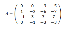
To find its inverse, we augment A to the identity matrix,

Then we bring this to row reduced echelon form, which is

Then our inverse would be

That’s all for section 7.6 (surprisingly, this section was shorter than most). Onto section 7.7!
No comments:
Post a Comment