7.7, where even and odd are deemed "remarkable"

Section 7.7 is entitled “Determinants.”

The question being answered this section is, “If we are given a matrix A, how do we know if its nullspace is nontrivial?” (I know; this is the question you’ve been asking since the beginning of nullspace.)

Before we answer this question, I’m going to warn you up front that the book just jumps into the idea of determinants pretty quickly. For example, the book literally says you’re supposed to recognize the determinant of a 2 × 2 matrix without any indication that we went over this. At least, from the sections I’ve had the pleasure (and displeasure) of reading in this journey through differential equations, I haven’t seen the determinant of a 2 × 2 matrix come up yet.

So I guess I’m trying to say that if you didn’t recognize determinants, even though the book apparently thinks you should, then that’s fine. If I wasn’t concurrently enrolled in a linear algebra class, I would be super confused about that idea as well.

Just for notation’s sake, the shorthand for “the determinant of A” is det(A). Now I feel much better about jumping into 7.7. At least, I feel less awkward about unfairly throwing unknown notation and equations and such things into your face.

Anyway, I’ll get onto the math words now.

Suppose A is a matrix where

Its determinant (which you’re just supposed to recognize) is ad – bc. Then A is nonsingular if and only if det(A) ≠ 0. In fact, this proposition is true for any square matrix.

If A is a square matrix, then the homogeneous equation Ax = 0 has a nonzero solution if and only if det(A) = 0. Then, to answer our original question, A will have a nontrivial nullspace if and only if the determinant of A is 0.

Moving on, for a 3x3 matrix A:

The determinant has the more complicated form det(A) = a₁₁a₂₂a₃₃ – a₁₁a₂₃a₃₂ – a₁₂a₂₁a₃₃ + a₁₂a₂₃a₃₁ – a₁₃a₂₂a₃₁ + a₁₃a₂₁a₃₂.

For a definition of determinant, let’s first look at one of the products when we looked at det(A) 3x3, let’s say a₁₃a₂₁a₃₂. The first subscripts are (1, 2, 3) and the second subscripts are (3, 1, 2). They’re the same 3 numbers, but they’re rearranged. If you look at all the products, you will see this is the case for all of them.

Determinants in higher dimensions also have this form. We need to notate some things before going to the definition.

“A permutation of the first n integers is a list σ of these integers in any order” (323). 

When we consider the 3x3 matrix, σ = (3, 1, 2) is a permutation of the first three integers.

Since a permutation is just a list of numbers, if we wanted to know how many permutations there are for 3 numbers, then we would have 6 different permutations for n = 3. (For any n, the number of permutations is n! (as in n factorial), so if you want to find the number of permutations, you could always do it that way. For n = 3, the number of permutations would be 3x2x1 = 6, which is what is in the book.)

These different permutations are (1, 2, 3), (1, 3, 2), (2, 1, 3), (2, 3, 1), (3, 1, 2), and (3, 2, 1). If you look back at our formula for the determinant of A, you’ll see these six different permutations are all present, with some minus signs thrown in.

So how do we know when to throw in a minus sign, and when to not throw in a minus sign? Well, when you’re looking at a permutation, say (3, 1, 2), then you have a number of interchanges you can make to transform this into a standard, ordered list of numbers. For example,

Then the book goes onto to say it’s remarkable that the number of interchanges needed for this operation is always even or always odd.

It’s…remarkable? I wasn’t aware the number of interchanges could be anything else besides even or odd.

 

Breaking news: the number of interchanges can either be even, odd, or bread. I can has math grant now?

Thus, the permutation is even if the number of interchanges is even, and the permutation is odd if the number of interchanges is odd. For example, (4, 2, 1, 3) would be even, while (4, 2, 3, 1) is odd. Conclusively, we will define a permutation σ

And now, the moment you’ve all been waiting for.

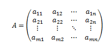
“The determinant of the matrix

is defined to be

where the sum is over all permutations of the first n integers” (324).

The actual definition isn’t going to be that helpful in calculating determinants, considering that the number of permutations for n = 4 is 4! = 24 permutations. That gets tedious and ridiculous very quickly. Therefore, we will almost never use the definition to compute a determinant.

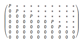
The exception to this rule is an upper or lower triangular matrix. (http://en.wikipedia.org/wiki/Triangular_matrix#Description) To save you from tedious work, you would use the summation and see that the determinant of an upper or lower triangular matrix is the product of its diagonal elements.

Some properties concerning determinants:

If A is a square matrix, and B is a matrix obtained from a multiple of one row to another of A, then their determinants will be equal. Similarly, if you swap two rows of A and call that resulting matrix B, then det(B) = -det(A). Finally, you obtained matrix B by multiplying a row of A by some constant c, then det(B) = c·det(A).

If matrix A has two equal columns, then its determinant is zero. Similarly, if A has two equal rows, then det(A) = 0.

Something neat about the transpose of A and A: det(A^T) = det(A).

Now, you might be wondering how you actually compute the determinant of a matrix if using the definition sucks. Well, you do something called expansion. You can expand on a row or a column. This is best shown by an example (and an exciting example, since I can make this one up and not experience deadly consequences. I mean, I can’t just make up an inverse example. The inverses of matrices go downhill very quickly when you just put random numbers wherever you feel like).

Before the example, let’s show some more summations.

If you want to expand on the ith row of a matrix, where 1 ≤ i ≤ n, then

If you want to expand on the jth column of a matrix, where 1 ≤ j ≤ n, then

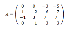
For example, consider the 3 × 3 matrix

Let’s expand on row and a column, just for the example’s sake.

If we expand on the third row, then we would have

If we expand on the second column, we would have

Notice we get the same answer for our row and column expansion. That’s nifty, right?

Finally, here are some more properties concerning determinants:

If A and B are n × n matrices, then det(AB) = det(A)det(B).

If A is a nonsingular matrix, then det(A^-1) = 1/det(A).

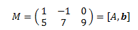
“A collection of n vectors x₁, x₂, … , x_n in Rⁿ is a basis for Rⁿ if and only if the matrix X = [x₁, x₂, … , x_n], whose column vectors are the indicated vectors, has a nonzero determinant” (328).

All right, that’s all chapter 7 has to offer you! The math is over now, so if you don’t want to read on about my struggles through this chapter (and why it was up so quickly), then just stop reading here and I’ll see you for chapter 8.

I’ll just let you know right now, I’m trying to get ahead of the game. As you already knew, I’m doing this blog only for the cookies (and for the selfless act of sharing said cookies with my differential equations class). I get points for each summary I post, and I get more points if my summary is released before we discuss that section in class. Well, I was very ahead once I had finished the summary for section 4.1, and that was exciting and all.

Then my instructor emailed me and told me that I was looking at the incorrect schedule and I needed to follow the weekly schedule. I shrugged my shoulders and moved onto doing the summaries for sections 6.1, 6.2, and 7.1. I was still ahead of the lecture, so I felt pretty good.

Then my instructor completely skipped over chapter 6 and he got dangerously close to catching up to my summaries.

It’s been slightly frustrating, and I’ve had a minor headache all week (since I’ve had homework, tests, and work/band things to attend to), but I’m hoping that by getting all of chapter 7 done this week, I’ll be ahead enough to not be rushing all of the time.

In other words, I’ve been rushing this week so I don’t have to rush ever again.

I’ll see you in chapter 8.

7.6 only allows the squarest of matrices.

Section 7.6 is entitled “Square Matrices.”

Square matrix has the same number of rows as columns (surprise, surprise!). This also is equivalent to a system of n equations with n unknowns. There are really interesting and lovely conclusions we can conclude about matrices that are square, and that’s basically what this section is all about.

Note: whenever I speak of the matrix A, A will always be a square matrix. In other words, A will be an n × n matrix. I’m going to try hard to write “square matrix A” whenever I speak of A, but if I don’t, I still want you to think of squares when I talk of A.

We should first think of when these types of systems can be solved for any and every choice on the right-hand side (think b in the equation Ax = b). If we can solve this system for any choice of b in Rⁿ, then we say the square matrix A is nonsingular. If we can’t, then the matrix is singular.

If we go through the motions of solving Ax = b, then we would create a matrix M that is the matrix A augmented with b, i.e. M = [A, b]. When we transform this augmented matrix into row echelon form, then we will get a matrix Q = [R, v], where R is the row echelon transformation of A. Q corresponds to the system Rx = v, where v is arbitrary. If A is nonsingular, then we must be able to solve Rx = v for any right-hand side we want. Therefore, A is nonsingular if and only if R is nonsingular.

Something else to note about the singularity of A is if R only has nonzero entries along its diagonal, then A will be nonsingular. Also, if A is nonsingular, then when we go to solve Ax = b, we will have a unique solution for x for every b we choose.

Now we’ll think a bit about the homogeneous equation Ax = 0. We know there is a nonzero solution for this system if there’s a free variable in the row reduced transform of A. If there’s a free variable, then there will be a zero in the diagonal entry of that column where the free variable resides. Because of this, the matrix must be singular for the system to have a nonzero solution.

Moving on, we’ll be speaking a bit about inverses now, so here’s a definition to start this discussion off:

“An n × n matrix A is invertible if there is an n × n matrix B such that AB = I and BA = I. A matrix B with this property is called an inverse of A” (320).

We will denote the inverse of A as A^-1. Something important to note about inverses is that a square matrix is invertible only if it’s nonsingular.

In order to find the inverse of the matrix A, you augment A to I, [A, I], and then row reduce that augmented matrix. You should get I augmented to some new matrix B, [I, B]. B is your inverse.

For example, consider the matrix

To find its inverse, we augment A to the identity matrix,

Then we bring this to row reduced echelon form, which is

Then our inverse would be

That’s all for section 7.6 (surprisingly, this section was shorter than most). Onto section 7.7! 

7.5: span and nullspace and base, oh my!

Section 7.5 is entitled “Bases of a Subspace.”

Let’s start with a definition: “If x₁, x₂, … , x_k are vectors in Rⁿ, we define the span of x₁, … , x_k to be the set of all linear combinations of x₁, … , x_k, and we will denote this set by span(x₁, … , x_k)” (308).

Allow me to remind you of the example I made up and did to show you what the span is of a matrix:

In this case,

Something similar to our properties of nullspace, we have some handy properties about span as well:

0. Assume x₁, … , x_k are vectors in Rⁿ and the set V = span(x₁, … , x_k).

1. If x and y are vectors in V, then so is their sum x + y.

2. If x is in V and a is a random number, then their product ax is also in V.

So these properties are basically the exact same for span and nullspace. There’s actually a special name for sets of vectors that have these properties: subspace. The exposition to subspace is that it must be a nonempty set and it must be in Rⁿ. So this is actually really awesome because if we have numbers a and b and we also have vectors x and y, and these vectors are in a subspace V. Then this means ax and by are in V, along with ax + by. This means that any linear combination of vectors in a subspace V will also be in V.

The zero vector is an element of every subspace. Also, a set with the single vector 0 can be a subspace. This subspace will also be denoted with a boldface zero, 0. Along with this really obvious subspace is the total space, Rⁿ, which is also a subspace. These two subspaces are known as trivial subspaces.

Assume V is a subspace of Rⁿ and V ≠ 0. Then there are vectors x₁, … , x_k such that V = span(x₁, … , x_k).

If V is indeed equal to this span, then we can say V is spanned by {x₁, … , x_k}. We can also say the set of vectors {x₁, … , x_k} spans V, or that {x₁, … , x_k} is the spanning set for V. It doesn’t matter how we say it; V is a set of all of the linear combinations x = a₁x₁ + a₂x₂ + … + a_kx_k, in which a_i­ can be any number. If we think of the coefficients as parameters, then our linear combination equation is a parametric equation for the subspace V = span((x₁, x₂, … , x_k).

So how do we know if one vector x is in a span of a set of other vectors? We have a method to follow concerning this question:

If you want to find out if x is in span(x₁, x₂, … , x_k), the you start by forming the matrix X = [x₁, x₂, … , x_k]. Then you solve the system Xa = x. You have two paths this road could lead you:

1. If there is no solution, then x is not in the span.

2. If a = (a₁, a₂, … , a_k)^T is a solution, then x is in the span.

Spanning sets for a subspace does not have to be unique. They don’t even need to have the same number of vectors. Just as an example, span(x₁, x₂) can equal span(x₁, x₂, x₃). However, we want to find a way to eliminate unneeded vectors from a spanning set. This want of ours leads to what is called linear dependence or independence. A set of vectors is linearly dependent if one or more of the vectors is unneeded to express the span. Here’s a formal definition for you concerning independence:

“The vectors x₁, x₂, … , x_k are linearly independent if the only linear combination of them that is equal to the zero vector is the trivial one where all of the coefficients are equal to 0. In symbols…” (312).

So if you want to determine if vectors (let’s call them x­₁, x₂, … , x_k) in Rⁿ are linearly dependent or independent, then what you want to do is form a matrix (let’s call it X) where the columns are your vectors x­₁, x₂, … , x_k. You’ll find null(X), and you’ll have two different sets of answers:

1. If null(X) = 0, then your vectors are linearly independent.

2. If you get a nonzero vector c = (c₁, c₂, … , c_k)^T, then you will have c­₁x₁ + c₁x₂ + … + c_kx_k = 0, which means your vectors are linearly dependent.

Remember, you find null(X) by reducing X to row echelon form and examining what is left over.

Moving onto a basis, which is the minimal spanning set (in a few words). If you have a set of vectors { x­₁, x₂, … , x_k} in a subspace V, they are a basis of V if and only if they have the following two properties:

1. The vectors span V

2. The vectors are linearly independent

If V is a subspace of Rⁿ, then V will have a basis. Furthermore, any two bases for V will have the exact same number of elements. These two facts brings us to a position where we can define the dimension of this subspace V. The dimension is the number of elements in any basis for V, but because V’s bases have the same number of elements, the dimension will be consistent. Hooray!

Something neat to note about Rⁿ and its dimension can be shown, but since this is a summary and I’m getting progressively lazy as this blog goes on, I will just give you the answer here and now (on the basis that you believe the things I am writing): dim Rⁿ = n. Also, something else to note about bases is that they are not unique. (The book stressed this note by putting it in italics, and so will I.)

If you want a good way of describing a subspace of Rⁿ, then you can simply provide a basis. Also, the dimension of the nullspace of a matrix is the number of free variables in the matrix. Neat, right?

I guess it’s time for an example since I’ve been spitting math words at you for a while and we should neatly tie everything together. I’m going to use a matrix from the book (and it’s also in reduced row echelon form, which is helpful in the context of time and space).

If we label each column by the respective variables x₁, x₂, x₃, x₄, and x₅, then the free variables are x­₂ and x₄ and x₅. We’ll set x₂ = s, x₄ = t, and x₅ = u, and we’ll then solve for our pivot variables (those being x₁ and x₃). In this case, null(C) would be parameterized by

Now we have to show that v₁, v₂, and v₃ are linearly independent. Remember, this is to determine what the basis of null(C) is. In order to do this, we will consider the linear combination of our vectors:

So if we want this linear combination to be equal to the zero vector, then we need those entries in the matrix to all equal zero. If we focus on the entries dealing with our free variables, then we see that c­₁, c₂, and c₃ are all equal to zero. Thus our linear combination is trivial, and we can also conclude that v₁, v₂, and v₃ are linearly independent. Our conclusion would then be that null(C) is the subspace of R⁵ with basis v₁, v₂, and v₃. Finally, because there are three vectors in the basis, this would make the dimension of null(C) equal to 3.

One final thing to leave you with:

If we are given the spanning set for a subspace, we can find a basis by eliminating unneeded vectors from the spanning set.

Okay, one more thing before I leave 7.5: If you’re slightly confused about what span is, I’ll provide some websites to possibly clear up any confusion. You could always read the book or go to class, though.

http://aleph0.clarku.edu/~djoyce/ma130/spanindep.pdf

http://en.wikipedia.org/wiki/Linear_span

I’ll see you when I see you.

7.4, or the section at which I realized that summarizing 3 of these a day really sucks.

Section 7.4 is entitled “Homogeneous and Inhomogeneous Systems.”

Just as a reminder, a homogeneous system has the form Ax = 0. Obviously, if we picked x to be the zero vector, then we would have a solution, since A0 = 0. Then we will call any solution x that isn’t 0 a nontrivial solution. So to be nontrivial, the vector must contain at least one nonzero component.

So, when you’re solving the system Ax = 0, you will go and augment A and 0 and bring it to row echelon form (or row reduced, either one). You will notice that the last column of your row echelon form will contain only zeroes. In other words, it didn’t change from the original zero vector it was. It’s not too difficult to see that this will always be the case. So it’s not really necessary to augment the coefficient matrix with the zero vector, but I suppose if you wanted to, I can’t stop you.

“The homogeneous system Ax = 0 has a nontrivial solution if and only if a matrix in row echelon form that is equivalent to A has a free column” (302).

“Any homogeneous linear system with fewer equations than unknowns has a nontrivial solution” (302).

So with inhomogeneous systems, our solution set will look vastly similar to stuff in section 7.2. We’ll have a particular solution to the inhomogeneous system Ax = b. We’ll denote this particular solution with a p. Our solution set for this system will have the form x = p + v, where Av = 0.

In other words, we’ll have the homogeneous solution (if the system was homogeneous, that is) and a particular solution together for the solution set for our inhomogeneous system.

This makes the homogeneous solution set very important, since we use it both for homogeneous and inhomogeneous solution sets. It’s so important, in fact, that it gets a special name. The nullspace of A is the set of all solutions to the homogeneous equation Ax = 0. It’s denoted by null(A).

A theorem concerning nullspace:

“The solution set of the inhomogeneous system Ax = b has the form

where p is any particular solution to the system Ax = b” (305).

Also, there are two properties of nullspace which are relevant:

1. If x and y are vectors in null(A), then x + y is also in null(A).

2. If x is in null(A) and a is a number, then ax is also in null(A).

Here’s an example concerning nullspace of a matrix:

If we name the variable for column one x₁ and for column two x₂, then x₂ is a free variable and we will give it the value x₂ = t. So then if we solved for x₁, then we would get x₁ = -5x₂.

Our variable t is just any arbitrary number of your choosing.

One final thing to leave you with for 7.4: a unit vector is a vector that has length one.

All right, that’s it for section 7.4. Onto 7.5!

Section 7.3 (row reduced madness)

Section 7.3 is entitled “Solving Systems of Equations.”

I’ll just start with the definitions and then show an example.

“The pivot of a row vector in a matrix is the first nonzero element of that row” (292).

So the first row, first column position (1), the second row, second column position (6), and the third row, fourth column position (16) are pivots.

“A matrix is a row echelon form (or just echelon form) if, in each row, that contains a pivot, the pivot lies to the right of the pivot in the preceding row. Any rows that contain only zeros must be at the bottom of the matrix” (293).

An example of a matrix in row echelon form:

Generally speaking, a matrix in row echelon form looks somewhat like this:

Where P represents some number that is the pivot of that row and the asterisks are arbitrary numbers.

If you want an example (video, steps, etc.): http://www.wikihow.com/Reduce-a-Matrix-to-Row-Echelon-Form

In order to get a matrix (and thus a system of equations) into row echelon form, we have three row operations we can perform:

1. Add a multiple of one row to a different row.

2. Interchange two rows.

3. Multiply a row by a nonzero number.

With these three row operations, you can literally (and I do mean literally) put any matrix into row echelon form.

If a matrix is in row echelon form, then there can be at most one pivot in each column. Then this column would be known as a pivot column, and the variable would be known as a pivot variable. The columns that are not pivot columns would be called a free column, and then the variable in that column would be known as a free variable. This is because you can assign any arbitrary value to this variable.

So then we’re down to a general formula to follow when trying to solve any linear system Ax = b. We first form the augmented matrix M = [A, b], then use row operations to reduce M to row echelon form. Once we have that simplified system, we can solve by assigning values to the free variables and then perform back-solving to find values for pivot variables.

So your next question might be, “How do we know when we don’t have a solution?”

This matrix basically says 0x + 0y = 8, or 0 = 8, and that’s not right. That’s not a thing that can happen in math. This system would be inconsistent and have no solutions.

The important thing to take from this is that a system is consistent if and only if it doesn’t have a pivot in the last column of its augmented row echelon form.

So if it’s possible, you can put your matrix in row reduced echelon form, in which your pivots are ones and the terms above your pivot variables are zeroes.

It’s your choice which form you want to bring your systems to. Row reduced requires a lot more work, but it’s super easy to solve. It’s really up to your tastes on what kind of work you want to do.

As a testimonial to you, the way this really makes sense is to work on examples, do the row operations, and watch the shapes form and the numbers work. You can find a hundred examples of matrices you can row reduce (or you can make your own, but they might become super gross super fast) and when you start to work on them, you’ll get better at noticing the patterns and understanding what needs to happen to make your life easier.

All right. I’ll see you in 7.4.

7.2, moar dimensions = moar fun

Section 7.2 is entitled “Systems of Linear Equations with Two or Three Variables.”

Let’s consider the equation 5x + 7y = 9. There will be a lot of different vectors that will satisfy this equation (i.e. solve it). The set of all of these vectors will be known as the solution set. In this case, the solution set would be a line in the xy-plane.

If we solve for y, we’ll get y = (9 – 5x)/7. This can be rewritten as

This equation is known as the parametric representation of the line modeled by our original equation. In this case, x is a free parameter, because any value of x will be a point on the line. For example, when x = 1, a point (1, 4/7)^T would be on the line. 

Generally, we would start at x = 0, and then that point would be called p. Then, for any value of x, we would add multiples of the vector v = (1, -5/7)^T.

(Reminder: The T is a transpose, and it’s just being used as a handy way to write vectors horizontally, despite their vertical traits.)

Time for our favorite words again!

Ax = b is said to be homogeneous if b is equal to the zero vector, which the book denotes by 0. If b is not equal to the zero vector, then the system is inhomogeneous.

And now for a definition:

“A line is Rⁿ is a set of the form

where p and v ≠ 0 are vectors in Rⁿ. [This equation above] is called a parametric equation for the line” (284).

The vector p is the point corresponding to t = 0. Our vector v gives us the direction of the line.

Now let’s look at two linear equations with two unknowns. Let’s consider the following equations:

5x + 7y = 9

x – y = 0

Separately, the solution sets for these equations are lines. Since we want the solution for both equations at the same time, then we’re looking for the line in which these equations intersect. Either there will be one point they intersect, or they will never intersect (because then they would be parallel).

We could solve this equation using algebra, by substituting x = y into our first equation and then getting answers. We would get 12y = 9, which would lead us to the new system of equations x – y = 0 and 12y = 9. We could add 12 times the first equation to the second and solve for x. This operation is called elimination (because our goal is to eliminate variables). Or you could just solve for y in our second equation and plug into the first equation to solve for x. Either way, you get the answer to be x = y = 9/12 = 3/4.

If we solved the second (i.e. last) equation first in our new system of equations and then solve the first equation, then we would be performing the method of back-solving. However, we usually have too difficult of equations and unknowns to simply back-solve and be on our merry way. We will usually use elimination to solve our equations.

Let’s rewrite our system in matrix notation:

If we define A as our coefficient matrix and b as the right hand side, we can rewrite this system as A(x y)^T = b. All of our information can be easily compacted into one larger matrix, called the augmented matrix.

We could also solve this matrix to look like our second set of equations, i.e. adding -5 times the first row to the second row. Then we would get

If the equations in a system are parallel, then they will have no solution. We call these systems inconsistent. We could also be presented with a system with equations that are multiples of each other. In this case, their solution sets would be the exact same. In conclusion of this, there are three and only three outcomes for solving a system of equations:

1. One point

2. A line

3. No solutions

Our first case happens often. The other two cases are called degenerate cases.

A bit more on homogeneous systems: They will always be consistent. So if you are presented with a homogeneous system, then you will never get “no solution” as the answer. The solution will either be the origin, or the line going through the origin.

If we were offered the line x + 2y – 4z = 5, then that equation is in three dimensions. We could solve this equation for x and get x = 5 – 2y + 4z. Then we would have the solution set be

Similar to the equation in two dimensions, this would be the parametric representation for a plane. In this representation, we have two free parameters: y and z. We would start at our point p = (5 0 0)^T and adding a linear combination of what is called v₁ and v₂. 

The formal definition:

“A plane in Rⁿ is a set of the form

where p, v₁, and v₂ are vectors in Rⁿ such that v₁ and v₂ are not multiples of each other. [The equation above] is called a parametric equation for the plane” (287).

If we were to look at two equations with three unknowns (which will make planes), then we know by geometry the solutions will have three possibilities:

1. The planes intersect in a line

2. The planes are the same plane and thus the solution set will be a plane

3. The planes are parallel and there will be no solution

In order to solve these equations, we shall use matrix notation and elimination. In some cases, we can eliminate some things and then make it possible to back solve. Then, in that case, we may be able to assign any value to a certain variable, say z, and then we can easily solve for numerical values for the other two variables, say x and y. In this case, we would call z a free variable and then we can set z = t (it’s the book way of saying, “hey, this can be any number”). This means the solution sets for planes will take on the following form:

This is just an example, but shows what our solution sets would look like.

For three equations and three unknowns, we will use matrix notation and elimination to prepare for back-solving. It sounds fairly simple, but it really can get messy. If you pick the right numbers, the answer can look gross. The solution sets for three equations with three unknowns will either be

1. One point

2. A line

3. A plane

4. No solution

If the equation is homogeneous, then the origin will always be a solution, which means homogeneous solutions will always have a solution. This means our possibilities for homogeneous systems are

1. The origin

2. A line though the origin

3.  A plane through the origin

Notice that we can have a single point as a solution for one, two, or three dimensions. This will look similar in any dimension. We also have lines in two dimension and lines and planes in three dimensions. They have common features that the book describes well:

“First, if we can move in a particular direction…we can move arbitrarily far in that direction. We can summarize this by saying that the set in infinitely long. Second, if there are two are two directions in which we can move, as in a plane, then we can move in any linear combination of those directions. We can summarize by saying that the solution set is flat. Finally, a line in the plane, or a line or plane in 3-space, does not take up much room. Both have negligible extent in most directions. We can summarize that by saying that the solution set is thin” (290).  

When we go into higher dimensions, we can’t really visualize it anymore and our intuition is lost. But we might think that these characteristic (long, flat, and thin) might also be used to describe solution sets in higher dimensions.

I guess we’ll find out when we go to section 7.3, but for now this is where we will end.

I’ll see you when I see you!

7.1, the section on the first week of the class I'm concurrently enrolled in: LINEAR ALGEBRA

Greeting from chapter 7! It is entitled “Matrix Algebra” and 7.1 is entitled “Vectors and Matrices.”

Just in time, too. I have a test in my Linear Algebra class this week (because I’m doubled up in math this semester).

In this chapter, we shall be dealing with systems of linear equations. Let us consider the equations

If we isolated the coefficients on the variables we would have what is called the coefficient matrix. Just to clarify, a matrix is a rectangular array of numbers, but we’re throwing out the rectangle part and using parentheses instead.

The numbers that appear in the matrix are called entries or components.

A column vector is a matrix that contains only one column. For instance,

The x vector is called the vector of unknowns and the b vector is just the right hand side of our system. We can rewrite our system into the compact form

In C, we have two rows and three columns. Generally, if we were to have m rows and n columns we would have

The size of A is (m, n) (rows first, and then columns). A is known as an m×n matrix.

A row vector is a matrix with only one row (similar to a column vector, except row version). Also, we might need to refer to our matrices by the number of elements. For example, x would be a 3-vector and b would be a 2-vector.

Vector is used in a lot of different places and usually means something different in each topic. Because of the variety of definitions that the term “vector” can take on, we have to be careful to determine which meaning we’re using. In this chapter of the book, a vector will always be an ordered list of numbers. However, watch out for when this isn’t a thing that happens in your life.

If we look back at our matrix C, we observe it can be thought as the two row vectors (3, 2, -6) and (5, -2, 7). We can also think of C as the three column vectors

Also, as a side note: 

Wikipedia proves to us that "vector" may be the most overused word in math and science.

Also, fictional characters named Vector? 

Anyway, back to the math. 

We can add matrices if and only if they are the same size. For example,

This would be called the matrix sum A + B.

The set of column vectors with n real entries is denoted by Rⁿ. If two vectors x and y are contained in Rⁿ (which is denoted by x, y ∈ Rⁿ, where ∈ means “element of”) then the matrix sum of x and y are also contained in Rⁿ.

Something useful to note about vectors (at least for this text) is that all vectors that are parallel are equivalent.

Equivalent. (Education.com)

Another handy operation that you can do on matrices is to is multiply a matrix by a constant. For example,

If x and y are vectors in Rⁿ, then a linear combination of these vectors is a vector of the form ax + by, where a and b are real numbers.

So back to our system from the beginning of this section summary: let’s rewrite our system as a linear combination:

The right-hand side of our equation will be denoted by b. Let’s rewrite our left-hand side of our system as the product of the coefficients C and a vector of our unknowns called x:

This means we can rewrite our system entirely as Cx = b, which may not mean a whole lot to you, but it’s kind of super exciting to me since I’m in a linear algebra class.

Here’s a definition for you (but first, some exposition):

Here’s a matrix we have already seen before:

Like last time, A is a matrix of m rows and n columns. Let’s define our column vectors a₁, a₂, …, a_n, which contain all the elements in the columns. So then we can show that A has these columns by writing A = [a₁, a₂, …, a_n].

Finally, let’s define the matrix x as a vector in Rⁿ.

“We define the product Ax of the matrix A [above this definition] and the vector x [less above this definition] to be the linear combination of the column vectors of A with the coefficients from the vector x.

Ax = x₁a₁ + x₂a₂ + … + x_na_n” (277).

So we’ll have m equations and n unknowns. This system can be written as

a₁₁x₁ + a₁₂x₂ + … + a_1n­x_n = b₁

a₂₁x₁ + a₂₂x₂ + … + a_2n­x_n = b₂

…

a_m1x₁ + a_m2x₂ + … + a_mn­x_n = b_m

Our right hand side of the system can be written as

Thus our general system can be rewritten as Ax = b. If Ax is defined, then number of columns in A must equal the number of rows in x.

Something that helped me with this is something I can possibly recreate using Paint:

I hope that kind of makes it better for you to understand.

Here’s a theorem about multiplication:

“Suppose A is an m x n matrix, x and y are in Rⁿ, and a is a number. Then

1. A(ax) = aAx

2. A(x + y) = Ax + Ay” (279).

Multiplication by A is called a linear operation. Also, no proof was given in the section (yes!). It’s fairly easy to prove these things using the definitions.

Multiplication of matrices A, B, and C is…

Associative: A(BC) = (AB)C

Distributive: A(B + C) = AB + BC or (B + C)A = BA + CA

However, it is a rare and wondrous occasion indeed for matrix multiplication to be commutative. This means it probably won’t be a thing to have AB = BA. You can make two matrices that can be multiplied both forwards and backwards (I would recommend a square matrix, like a 2 x 2 or a 3 x 3). In any event, unless you choose the zero matrix (zeroes in every place) then you will find that you’re either really amazing at picking random numbers or the commutative properties don’t happen often for multiplying matrices.

Here’s the identity matrix:

As you can see, there are ones on the diagonal and zeroes every other place. Something cool to note about the identity matrix is that Ix = x for every vector x. This means that IA = A and BI = B.

One more thing to leave you with concerning this section is the transpose of a matrix.

Here’s our matrix A:

Here’s the transpose:

So you just flip the matrix along its main diagonal. Here’s an example:

Something nice about this is that a matrix with m rows and n columns will have a transpose of n rows and m columns.

Okay, that’s about it for 7.1. Just to let you know, we have 6 more sections of chapter 7. I’ll see you when I see you.