5.7 - the last end of a chapter you'll ever see D':

Section 5.7 is entitled “Convolutions.”

Let’s review a little bit of what we have learned in the past:

(It’s probably near the end of this epic mashup: http://differentialequationsjourney.blogspot.com/2013/11/52-54-where-you-refine-your-powers-of.html)

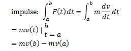
At the end of our summary through 5.6 (i.e. http://differentialequationsjourney.blogspot.com/2013/11/56-last-second-to-last-section-maybe.html) we talked about something called the unit impulse response function. Since the denominator of our Laplace transform is the characteristic polynomial of our second order differential equation, we can rewrite that Laplace transform as

In this case, E(s) is the Laplace transform of the unit impulse response function e(t) for our differential equation. So now we can find a solution to the differential equation by taking the inverse Laplace transform of our rewritten Laplace transform, i.e.

Let’s now look at a proposition:

“Suppose that f and g are functions of exponential order. Suppose that ℒ(f)(s) = F(s) and ℒ(g)(s) = G(s). Then

Note that the choice of the variable of u is merely a choice. The variable of integration could be anything, in theory, since the resulting expression is a function of t at the end of the day.

Now, let’s define something:

“The convolution of two piecewise continuous functions f and g is the function f * g defined by

The means we can rewrite what we said in the proposition as

Now, let’s look at a theorem:

“Suppose f and g are functions of exponential order. Then

Here’s another theorem:

“Suppose f, g, and h are piecewise continuous functions. Then

1. f * g = g * f

2. f * (g + h) = f * g + f * h

3. (f * g) * h = f * (g * h)

4. f * 0 = 0” (235).

(Note: three theorems separate us from the end of this blog.)

Now, we want to think in terms of the general solution to our original initial value problem (which I’ll state once again because why not and also because we’re going to make it a little more general):

Let’s take a look at the theorem that will answer all our questions:

“The solution to the initial value problem [above] can be written as

[where y_s(t) is the state-free solution and y_i(t) is the input-free solution]. If e(t) is the unit impulse response function for the system, then the state-free response is

and the input-free response is

Let’s now think of properties of the convolution. For one thing, f * 1 is NOT equal to f. This means, unlike a lot of other subjects in mathematics, the function 1 is not the identity for the convolution product. Here’s a theorem for the identity:

“Suppose f is a piecewise continuous function. Then

Allow me to take the time right now to remind you that δ₀ is the delta function when p = 0 (http://differentialequationsjourney.blogspot.com/2013/11/56-last-second-to-last-section-maybe.html).

Something nice about this result is that

Finally (and by finally, I mean for the final time in this blog), here’s a theorem:

“Suppose f and g are piecewise differentiable functions. Then

Here are some websites concerning the interesting phenomenon of convolutions:

http://en.wikipedia.org/wiki/Convolution (This will probably be more confusing than helpful but I’m adding it anyway)

http://faculty.atu.edu/mfinan/4243/section76.pdf (This contains more problems for you to work out than examples, but that’s okay, I suppose)

http://tutorial.math.lamar.edu/Classes/DE/ConvolutionIntegrals.aspx

http://www.swarthmore.edu/NatSci/echeeve1/Class/e12/Lectures/ImpulseConvolution/ConvolutionExamples.pdf (This contains quite a few graphs. There were no graphs in the section in the book so this might be more confusing than helpful.)

All right, that’s it. My teacher told me to not worry about chapter 10, so I won’t.

Wow, this is weird. I’m finishing something that has taken up so much time in my semester. This is bittersweet. I like the idea of not having to worry about this blog anymore, but I kind of enjoyed it in a no-one-reads-this-anyway-so-I-don’t-need-to-feel-pressured sort of way.

The journey is over summary-wise but not semester-wise. I still have a couple of weeks before this semester is over so we’ll see what happens.

Goodbye, math blog. (For now.)

5.6, the last second-to-last section (maybe) (hopefully) (I don't actually care if it is)

Section 5.6 is entitled “The Delta Function.”

So guys. This is a pretty theorem-heavy section. In fact, I don’t quite count it as a section I had to summary because all I have to do is quote all the definitions and theorems and be on my merry way. Sure, it takes some effort on my part, but it’s a really nice section to end on until at least Friday (once my test is dead and gone).

Let’s start with a definition of what we mean by the impulse of a force:

“Suppose F(t) represents a force applied to an object m at time t. Then the impulse of F over the time interval a ≤ t ≤ is defined as

In physics terms, the impulse is the change in momentum of a mass as a force is being applied to it during a certain time interval (in this case, a ≤ t ≤ b). If we recall a simpler time (in chapter 2, I believe) (http://differentialequationsjourney.blogspot.com/2013/08/section-23-words-and-then-numbers.html) when we first thought of Newton’s Second Law, we know F = ma = m*dv/dt. Therefore we can rewrite impulse as

If you know even a little bit about physics, you’ll recognize the form mv as the function of momentum. Thus impulse really is the change of momentum on an interval of time.

Now let’s consider a force of unit impulse over a short interval of time, which is what we’ll recognize as a piecewise continuous function. We can also translate this into terms of the Heaviside function:

The interesting thing about this function is that for any epsilon, there will be an area that is a rectangle (since it’s a piecewise function that has constants as its functions) and the area of that rectangle will always be 1. So if we want a model of this kind of force (which is sharp and instantaneous) as a time t = p, then we can take the limit as ϵ goes to zero.

Now let’s define something:

“The delta function centered at t = p is the limit

When p = 0, we will set δ = δ₀” (229).

Something interesting about this function is that it’s not even a function. Mathematicians call it a generalized function or a distribution.

Let’s look at two theorems and a corollary:

“Suppose p ≥ 0 is any fixed point and let φ be any function that is continuous at t = p. Then

In particular, this theorem can be used to compute the Laplace transform of the delta function centered at p” (230).

“For p ≥ 0, the Laplace transform of δ_p is given by

Finally, the case when p = 0 is important (and slightly obvious), but ℒ(δ₀)(s) = 1.

Finally, here’s a definition and a theorem:

“The solution e(t) to the initial value problem

is called the unit impulse response function to the system modeled by the differential equation” (230).

“Let e(t) be the unit impulse response function for the system modeled by the equation

The Laplace transform of e is the reciprocal of the characteristic polynomial P(s) = as² + bs + c.

That’s it for 5.6. I kind of wish I wanted to just finish the chapter and get 5.7 up tonight, but I don’t. I have other homework I need to get started since I have limited time to study for my test. Yay obligations!

I’ll see you in 5.7 (in a good while. I hope you enjoy your break as much as I will enjoy mine).

5.5, or more of piecewise-ness

Section 5.5 is entitled “Discontinuous Forcing Terms.”

We’ve already looked at sinusoidal forcing terms. It’s high time we look at piecewise continuous forcing terms.

Specifically, we’ll be looking at two kinds of functions: the interval function and the Heaviside function.

Some properties about the Heaviside function:

Also, the interval function H_ab(t) can be described using the Heaviside function:

You can also describe piecewise functions in terms of the Heaviside function; for example, if we consider

We have the intervals 0 ≤ t < 4, 4 ≤ t < 6, and 6 ≤ t, so we’ll use the interval functions H₀₄, H₄₆, and H₆:

Now, for the Laplace transform of the Heaviside function:

In particular, we have ℒ(H)(s) = 1/s. Also, for the interval function H_ab = H_a – H_b:

A proposition for you: “Suppose f(t) is piecewise continuous and is of exponential order. Let F(s) be the Laplace transform of f. Then, for c ≥ 0, the Laplace transform of H(t – c)f(t – c) is given by

Back to our original example: We had translated that piecewise function to 3H(t) – 8H(t – 4) + 5H(t – 6) + e^7-tH(t – 6) and now we want to find the Laplace transform. The first three terms can be handled with that handy proposition, and the last one can be rewritten as H(t – 6)e^-(t-6)×e, and we can use that table from one of the previous sections (http://differentialequationsjourney.blogspot.com/2013/11/52-54-where-you-refine-your-powers-of.html) and this proposition to take care of it. Thus we have

Another proposition for you: “Suppose that f(t) is piecewise continuous and is of exponential type. Suppose that F(s) = ℒ(f)(s). Then

Finally, let’s talk about periodic functions. A periodic function is one that has a repetitive pattern (as you can imagine). The formal definition says that “f is periodic with period T (or T-periodic) if f(t + T) = f(t) for all t” (222). Sinusoidal functions are periodic, just for an example. Another example of a periodic function is called a square wave. From a geometric perspective, if the function f is a T-periodic function, then it repeats every interval of T. For this type of function, we can define the window of f as

Finally (finally), here’s a proposition for you: “Suppose f is periodic with period T and piecewise continuous. Let F_T(s) be the Laplace transform of its window f_T. Then

That’s it for 5.5! I was planning on combining 5.5, 5.6, and 5.7 but I just don’t have the time to get them all written up. I’m not on a time crunch or anything (quite the opposite, actually), but I really do want to get them all up by Sunday. If I did that, I would only have those two sections of chapter 10 (if that) and I wouldn’t be thinking of them after my test.

Speaking of which, there shall be no summaries up next week. This is because of my differential equations test.

I’ll see you in 5.6. 

5.2-5.4, where you refine your powers of propositions and partial fractions

Section 5.2 is entitled “Basic Properties of the Laplace Transform.”

This section is just a ton of propositions. Seriously, I could leave the summary at just that and I think everyone would agree that I have successfully summarized this section.

Oh, well. Onto ALL of the definitions! (Note: Since this is just a summary blog, I will not be supplying the proofs. I shall be milking the “it’s just a summary” excuse quite a bit for this section.)

“Suppose y is a piecewise differentiable function of exponential order. Suppose also that y’ is of exponential order. Then for large values of s,

where Y(s) is the Laplace transform of y” (197).

The point of this proposition is that now it’s relatively easy to find the derivative of a function. Now, you could throw out really easy functions with really easy derivatives (f(t) = t, f(t) = sin(t), f(t) = e^t, etc.) but for other functions, it might be easier to use this method.

“Suppose that y and y’ are piecewise differentiable and continuous and that y” is piecewise continuous. Suppose that all three are of exponential order. Then

where Y(s) is the Laplace transform of y. More generally, if y and all of its derivatives up to order k-1 are piecewise differentiable and continuous, and y^(k) is piecewise continuous, and all of them have exponential order, then

“Suppose f and g are piecewise continuous functions of exponential order, and α and β are constants. Then

The point is that the Laplace transform of a linear combination of functions can be computed by taking the Laplace transform of each term separately and then adding up the result” (199).

“Suppose f is a piecewise continuous function of exponential order. Let F(s) be the Laplace transform of f, and let c be any constant. Then

“Suppose f is a piecewise continuous function of exponential order, and let F(s) be its Laplace transform. Then

More generally, if n is any positive integer, then

So that’s it for section 5.2. I told you it was a lot of propositions.

Section 5.3 is entitled “The Inverse Laplace Transform.”

Before we talk about the inverse, we need to introduce a theorem to clear up any concern.

“Suppose that f and g are continuous functions and that ℒ(f)(s) = ℒ(g)(s) for s > a. Then f(t) = g(t) for all t > 0” (203).

In other words, we have yet another uniqueness theorem to tuck underneath our belts. Also, I couldn’t prove this to you even if I had the proof in front of me, because apparently the proof goes beyond the scope of the book. That both terrifies me and excites me (I wouldn’t be a good physics major if I wasn’t curious about everything, now would I?).

Anyway, onto the definition:

“If f is a continuous function of exponential order and ℒ(f)(s) = F(s), then we call f the inverse Laplace transform of F, and write

Here’s a Paint picture to help clear up any confusion (and also for any visual learners out there):

A proposition for you: “The inverse Laplace transform is linear. Suppose that ℒ^-1(F) = f and ℒ^-1(G) = g. Then for any constants a and b,

Also, here’s a table of some common Laplace transforms (which you can probably find in a million other places here on the internet, but here it is nonetheless):

In order to complete this section, I have to bring back something I am not particularly fond of: partial fractions.

If you want a refresher on the subject (I know I did), here are a couple of websites for you (personally, I’m not very fond of the Wikipedia article on the subject. I’d say to go for the one with pretty colors): http://en.wikipedia.org/wiki/Partial_fraction_decomposition, http://www.purplemath.com/modules/partfrac.htm, http://www.mathsisfun.com/algebra/partial-fractions.html

The reason why this is brought up is because with the power of partial fractions, we can compute the inverse Laplace transform of most rational functions. I’ll include one example just to show you how it’s done!

That’s it for section 5.3! As long as you remember partial fractions, you really should be golden.

Section 5.4 is entitled “Using the Laplace Transform to Solve Differential Equations.”

In other words, the previous sections were more preface than anything else. They were merely the building the blocks for you to get to this section. Hooray! With your newfound power of partial fractions, Laplace transforms, inverse Laplace transforms, and propositions, you’ll be able to solve differential equations (with initial conditions, too)!

You can also solve higher order differential equations as well (say, order 4), and those equations are handled pretty much the same way. Anyway, here’s an overview of the method:

We’ll be looking at the following initial value problem:

We apply Laplace transform to this, where Y(s) = ℒ(y)(s):

If y is a solution to the initial value problem to our original differential equation, then ℒ(ay” + by’ + cy) = ℒ(f) = F. We can substitute this into the equation above and solve for Y. This means that

Something interesting to note about that final equation is that the denominator is the characteristic polynomial of our original differential equation.

Finally, two definitions:

Suppose y_s is the solution of

Also, suppose y_i is the solution of

Notice that although y_s has initial conditions equal to zero, it has the same forcing term (i.e. f(t)) as our original differential equation. This is referred to as the state-free solution. On the other hand, y_i is the solution to a homogeneous equation, but it has the same initial conditions. This is referred to as the input-free solution. From our previous derivations, we have

It’s pretty plain to see that Y can be written as Y = Y_s + Y_i, and from this we can see that y = y_s + y_i. Therefore, any initial value problems can be written as the sum of its state-free and input-free solutions.

And that’s it for 5.4 and the evening! 5.5 is going to be a bit more tedious than I previously thought, but it’s not that long of a section. I have a test in this class coming up fairly soon, and thus I would like to go about the test week the same way I did last time. I’d like to not have to summarize new material whilst trying to remember the old material.

Finally, a for-your-information type of thing, there are 3 more sections to cover in chapter 5, and then I’m going to ask about chapter 10 (in which we might look at the first two sections). If my teacher says I should summarize those as well, that means we have 5 more sections together before I’m off to bigger and better things (i.e. going onto Tumblr and spending these hours there).

Perhaps I will write an epilogue to this epic journey, just as a closer. We’ll cross that bridge when we come to it, though.

I’ll see you when I see you.