5.6, the last second-to-last section (maybe) (hopefully) (I don't actually care if it is)

Section 5.6 is entitled “The Delta Function.”

So guys. This is a pretty theorem-heavy section. In fact, I don’t quite count it as a section I had to summary because all I have to do is quote all the definitions and theorems and be on my merry way. Sure, it takes some effort on my part, but it’s a really nice section to end on until at least Friday (once my test is dead and gone).

Let’s start with a definition of what we mean by the impulse of a force:

“Suppose F(t) represents a force applied to an object m at time t. Then the impulse of F over the time interval a ≤ t ≤ is defined as

In physics terms, the impulse is the change in momentum of a mass as a force is being applied to it during a certain time interval (in this case, a ≤ t ≤ b). If we recall a simpler time (in chapter 2, I believe) (http://differentialequationsjourney.blogspot.com/2013/08/section-23-words-and-then-numbers.html) when we first thought of Newton’s Second Law, we know F = ma = m*dv/dt. Therefore we can rewrite impulse as

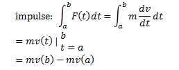
If you know even a little bit about physics, you’ll recognize the form mv as the function of momentum. Thus impulse really is the change of momentum on an interval of time.

Now let’s consider a force of unit impulse over a short interval of time, which is what we’ll recognize as a piecewise continuous function. We can also translate this into terms of the Heaviside function:

The interesting thing about this function is that for any epsilon, there will be an area that is a rectangle (since it’s a piecewise function that has constants as its functions) and the area of that rectangle will always be 1. So if we want a model of this kind of force (which is sharp and instantaneous) as a time t = p, then we can take the limit as ϵ goes to zero.

Now let’s define something:

“The delta function centered at t = p is the limit

When p = 0, we will set δ = δ₀” (229).

Something interesting about this function is that it’s not even a function. Mathematicians call it a generalized function or a distribution.

Let’s look at two theorems and a corollary:

“Suppose p ≥ 0 is any fixed point and let φ be any function that is continuous at t = p. Then

In particular, this theorem can be used to compute the Laplace transform of the delta function centered at p” (230).

“For p ≥ 0, the Laplace transform of δ_p is given by

Finally, the case when p = 0 is important (and slightly obvious), but ℒ(δ₀)(s) = 1.

Finally, here’s a definition and a theorem:

“The solution e(t) to the initial value problem

is called the unit impulse response function to the system modeled by the differential equation” (230).

“Let e(t) be the unit impulse response function for the system modeled by the equation

The Laplace transform of e is the reciprocal of the characteristic polynomial P(s) = as² + bs + c.

That’s it for 5.6. I kind of wish I wanted to just finish the chapter and get 5.7 up tonight, but I don’t. I have other homework I need to get started since I have limited time to study for my test. Yay obligations!

I’ll see you in 5.7 (in a good while. I hope you enjoy your break as much as I will enjoy mine).