Section 2.3: Words and then Numbers

Section 2.3 is entitled “Models of Motion.”

This section has quite a bit of words about history and physics and such. If you’re here for the numbers, you’re going to have quite a bit of exposition to get through. I’d apologize, but history is cool and physics is cool and together they are awesome.

The study of motion has been a thing for thousands of years. Humans are fascinated particularly by the motion of planets, and have tried to model their motion for years (as far back as the Babylonians, who made the first recorded observations regarding planetary motion).

Greek astronomers Hipparchus and Ptolemy believed the earth was the center of the universe and that everything (including but not limited to the sun, the moon, and other planets) revolved at constant velocities in circular paths around the earth. Then again, pretty much everyone believed the earth was the center of the universe. Well, everyone except Aristarchus, it seems.

My interpretation of their confrontation. These would be their exact quote, of course.

As math got better, Hipparchus and Ptolemy realized the circular paths part of their theory wasn’t true. To account for this, they developed epicycles, which are smaller circles around the larger circle. The center of the smaller circle rotated in a circular path, while the other planets rotated in the smaller circle. So the planets would move around the epicycles as the epicycles moved around the earth.

E means earth. P means planet. C means center of smaller circle.

The next major improvement came in the 16th century, when Copernicus stated the earth was not the center and rather the sun was the center. This was a major change in the way people thought in that time, but it made the epicycle calculations much easier to do so I guess it all worked out in the end.

In 1609, Tycho Brahe (the most fun physicist name to say, if I do say so myself) made observations about the motion of planets and Johannes Kepler created the three laws of planetary motion:

“1. Each planet moves in an ellipse with the sun at one focus.

2. The line between the sun and a planet sweeps out equal areas in equal times.

3. The squares of the periods of revolution of the planets are proportional to the cubes of the semi-major axis of their elliptic orbits” (38).

Coincidentally, Tycho Brahe also had one of the more impressive moustaches (Wikipedia) 

The great thing about Kepler’s laws was that there was no more need for epicycles. Also, the idea that planets and moons and such interstellar bodies were traveling at a constant speed were thrown out as well.

Our next stop on the history of astronomy train is Newton, who made three major advances when it came to planetary motion. First, he created calculus, which helped to derive and thus validate Kepler’s laws. Second, he created the laws of mechanics. In particular, we’re talking about his second law (force is equal to mass multiplied by acceleration), because then the study of motion could be simplified down to differential equations. Third, he postulated the universal law of gravity, which mathematically described gravity.

In 1919, Einstein proposed the theory of relativity, which explained gravity as the result of the curvature of four-dimensional space-time.

Gravity makes sense now...I think. (NASA)

In the 20th century, physicists have realized there are four fundamental forces of the universe: gravity, the strong nuclear force, the weak nuclear force, and the electromagnetic force. However, physicists strongly believed all of these forces are unified. Quantum mechanics links three of the forces (minus gravity), and there is a disconnect between the way relativity explains the universe and how quantum explains the universe. I could create an entirely different post about the differences and the way each explains the universe, but this is math and I shall continue on.

Recently (but not recently, since we have the M-theory now), some physicists have created the string theory as a way to unify relativity and quantum mechanics. The shorthand version of string theory says that particles in the universe act as strings that move in 10-dimensional space time. (M-theory postulates 11 dimensions, but we’re not going to overturn that rock.)

Because 4 dimensional space-time is too mainstream. (particlecentral.com)

However, at this point string theory (superstring theory, M-theory, what have you) cannot be validated. Physicists are working on an experiment to test this theory, but for now we will just have to wait.

*

The previous history lesson presented about six mathematical models or theories of planetary motion (I counted, but I don’t want to recount and list them for you, so just take my word for it). With each updated model, there was a more general application for the motion of planets. This is an elaborate example of what should happen whenever a mathematical model is created or used – when we become better educated, we should change the theories to make them better.

Looking specifically at Newton’s theory of motion, we’re going to dive into numbers now. At this point, the book is limiting us to one dimensional motion. Hey, at least they didn’t just throw us in the metaphorical pool of ten-dimensional space time math problems and say, “Swim or die.”

I don't know about you, but I'd probably drown.

We’re going to look at a very general example of a ball bouncing straight up and down in the air.

You can tell this is going to be exciting because the background is yellow.

Let x be the distance between the ball and Earth’s surface. Let m be the mass of the ball. From first semester calculus/physics, we know that the velocity is the first derivative of the distance and acceleration is the second derivative of distance (and thus the first derivative of velocity). Newton’s second law says the force on the ball is equal to its mass times the acceleration it is falling at. Since the ball is under the influence of gravity, the equation is as such:

where g is the gravitational constant. Knowing all these things, Newton’s second law on the ball becomes:

Since this is a differential equation, this can be solved. I’m not going to solve it step-by-step but instead show you the answer:

The initial velocity is v_0 and the initial height is x_0.

With this example, we took on the assumption that gravity was the only force acting on the ball. In real life, this isn’t true. There are quite a few forces acting on a ball that is falling to earth. We’re going to talk about air resistance now.

Here are three facts about air resistance:

1. If the velocity is zero, there is no motion and that means there is no resistance.

2. Resistance will always act opposite to the direction of an object’s motion. This means resistance will have a sign opposite of velocity.

3. Resistance is very complicated and no one law can describe all cases. There are many cases (because this is reality, where stuff changes every day).

You can quote me. I'm deep.

For now, we’re just going to focus on two different cases. For these two cases, we’re going to solve a differential equation, look at terminal velocity (more explanation in a second), and solve for the displacement. There’s quite a bit of math involved (to balance out the words at the beginning, I suppose).

Case 1: r is a positive constant

Forces can be superimposed, so our equation starts off as the following:

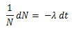
This equation is separable and thus solvable. Skipping over those steps (do it yourself for the practice, I suppose), the solution is

C is just a constant. Now, if we look at the limit as time goes to infinity, we are left with –mg/r, which is what we call terminal velocity. This basically means that if a colored pencil was dropped from the top of a building, at some point the pencil will stop accelerating and will fall at a near-constant velocity based on its mass and air resistance.

Finally, let’s solve for displacement:

A is another constant due to the integration required to find displacement.

Case 2: magnitude of the resistance is proportional to the square of the velocity

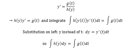
In the language of math, our second case is as follows:

With Newton’s law, this becomes

The book uses tricky calculus to solve this by substituting v and t for other things. If you believe the book (and if you believe me), then I’m going to skip these steps.

The solution is

Do you vaguely understand the situation, now?

As time goes to infinity, the terminal velocity is modeled as

Because of the monster of a solution above, integrating to find displacement would just be crazy.

(Caption: They know what they’re talking about.)

Instead, we’re going to use the chain rule.

That is all for this section, ladies and gentlemen! I’m trying to have fun with the blog because for the most part, math summaries can be pretty dull. I hope you’re enjoying it as much as I am.

For more information about air resistance, visit this page. It looks legit: http://physics.info/drag/

Section 2.2: Separable Equations and Tricky Calculus

Section 2.2 is entitled “Solutions to Separable Equations.”

Let’s start with the definition of a separable equation. Surprise, surprise! This type of equation can be rewritten with its independent and dependent variables separated from one another.

The book uses the following equation as their example (so I’m going to use this example as well):

N is a function and lambda is a constant. This equation is use in problems involving the half-life of radioactive elements. In this example, N is the dependent variable and t (which stands for time) is the independent variable.

Now, I shall demonstrate the art of separating equations.

Now we can go one of two ways: the physics way or the tricky calculus way.

My teacher provided the following diagram to explain why we should go the physics way:

Note: not his diagram, rather my crappy Paint version of his diagram

This is what I saw:

(Note: Just kidding. But really physics is easier to understand, never mind legitimacy)

In all reality, the tricky calculus way isn’t that bad. It’s just easier to do the physics way because that’s just how physics rolls.

Now, we separate the “N” variables from the “t” variables. Note that there are no t variables on site (besides the dt) but lambda is included in the “t” variables because it’s a constant.

And we integrate!

This type of equation is also known as an exponential function, because the solution contains an exponent.

This is the basic method for solving separable equations:

1. Separate variables

2. Integrate

3. Solve for the dependent variable.

Note that separable equations will either take the form of

Adding (or subtracting) is not separable. Tricky calculus cannot help us save the day :(

Here’s a definition from the book (throwback to last section):

General solution: “A family of solutions depending on sufficiently many parameters to give all but finitely many solutions” (30).

In other words, a general solution might not give a solution to every initial value problem thrown its way (for example, when division by zero is a factor).

Here’s another definition (and another example of a separable equation):

Newton’s Law of Cooling: “The rate of change of an object’s temperature is proportional to the difference between the temperature and the ambient temperature” (31).

By the way, the example given to show Newton’s Law of Cooling involves a can of beer. Is this is a college textbook or what?

The unsolved separable equation for Newton's Law of Cooling is as follows:

A is the ambient temperature (for instance, room temperature or outside temperature). T₀ is the initial temperature of the object. The constant k can be solved for and then you’re all good to go with solving for lots of things!

Here’s a link to someone who actually took the time to solve the Newton’s Law of Cooling equation with steps and stuff: http://www.math.wpi.edu/Course_Materials/MA1022A96/lab2/node5.html

Something to note about separable equations is that sometimes solving after integration is very difficult, and sometimes not even the trickiest of calculus can simplify our solution to just one dependent variable.

For example, y = 5x + 2 is simplified.

For non-example, the following equation cannot be simplified:

Some definitions for you:

Explicit: formula as a function in terms of the independent variable (our example shows this).

Implicit: the opposite of explicit. Our non-example shows this.

Finally, I shall show you why the separation of variables step (i.e. the physics way of solving separable equations) works.

 

In all reality, validation is never a bad thing.

Nevertheless, say we start with the following equation:

Note this is very similar to the h(y)dy = g(t)dt step we do in the physics version. 

Mathematics deems this step to be meaningless (since dy and dt by themselves don’t make much sense without integrals). I understand and appreciate the validation of the physics way, and I hope you do as well.

Definitions, Derivatives, Integrals, and First Order Nonsense

           

As a side note, I use quotes taken directly from the book sometimes. You may not think that is the consistency of a summary, but I think the best summaries involve the words of people who really know what they’re talking about. These three gentlemen who wrote my math book have far more experience and wisdom about differential equations than I do. Therefore I think I am just in my actions in using quotes direct from the text.

Before I begin with summaries and such, I thought I’d share with you my thoughts about the most serious paragraph in the preface, entitled “Mathematical Rigor.”

First of all, I knew this was going to be super serious when I read the sentence “Mathematical ideas are not dodged.” Don’t ignore the ideas behind math, people! They’re super important. Also, the word “dodged” seems like a British word to me (someone else has to feel this way as well!). This makes me think that one or more of the authors must be British. I looked up the authors of my textbook and I now know that Polking and Boggess are not British but I can’t find any birth information on Mr. Arnold. He works in California so I can’t just assume he’s British. My hypothesis has failed and I now turn to the “they’re very smart gentlemen” hypothesis.

Anyway, this paragraph really sprinkles in the emphasis behind understanding the theorems and proofs working in the shadows of the textbook. Note: “The authors believe that proof is fundamental to mathematics, and that students at this level should be introduced gently to proof as an integral part of their training in mathematics” (xii). I’m fine with the fact that these authors are humble enough to refer themselves in the third person, but I also think they’re pushing math pun with “integral” and that’s just amazing.

Anyway, onto the sections.

Chapter 1 is entitled “Introduction to Differential Equations.” Section 1.1 is entitled “Differential Equation Models.”

It’s an introduction to the book, so it’s just introducing what the book is going to teach us, in a sense. The first four paragraphs before the first section state there shall be quite a few examples from physics and chemistry and other subjects that include and are related to differential equations. There is also an emphasis of the importance of differential equations and the level of usefulness in real life. Note: “If it were not true that differential equations were so useful, we would not be studying them…” (1).

In the first section, there are a lot of examples of how differential equations are used in everyday life. The topics of study for differential equations listed are mechanics, population models, pollution, and personal finance, along with others (aptly titled “other examples”). My personal favorite is mechanics, because Isaac Newton is involved and so is physics. He was key in the development of differential equations because he just so happened to invent calculus and a lot of classical physics. There could be hundreds of examples for differential equations (including but not limited to electricity and magnetism) but the major point is that this kind of modeling the world due to its reliability and precision.

Section 1.2 is entitled “The Derivative.”

The section starts off with the question, “What is a derivative?” Five answers are given: the rate of change of a function, the slope of the tangent line to the graph of a function, the best linear approximation of a function, the limit of the quotients, to which the following function was given:

and the final answer to the question “What is a derivative?” was given in a table of derivatives, which included the simple ones such as the constant and the cosine of x.

When the derivative is referred to as the rate of change, it is also known as the modeling definition of the derivative. When the derivative is referred to as the slope of the tangent line, it is also known as the geometric definition of the derivative. When the derivative is referred to as the best linear approximation, it is also known as the algebraic definition of the derivative. When the derivative is referred to as the limit of difference quotients, it is also known as the limit quotient definition. And, of course, the formulaic definition is the list of formulas.

Crappy Paint version of the slope of the tangent line (geometric definition)

Section 1.3 is entitled “Integration.”

Just like the last one, this section starts off with a question. This time, the question is “What is an integral?” The following three answers are given: the area under the graph of a function, the anti-derivative, and a table of integrals.

The area under the graph is also known as the definite integral. It is the most fundamental definition of the integral.

The anti-derivative is synonymous with the indefinite integral. There’s a handy little equivalence in the book that states that if f is continuous,

Also, the fundamental theorem of calculus is back! It’s what connect

s the definite and the indefinite integral. Of course, it is stated that if f prime = g, then

The authors state that although the table of formulas is a handy skill to have, it does not lead to a deep understanding of integration. However, the authors go on to state all the approaches (the area, the anti-derivative, and the formulas) are important. But the authors also stress the importance of finding anti-derivatives, and so do I. When we move onto solving differential equations (i.e. in the next chapter of the book) finding anti-derivatives is a crucial part for solving them.

When solved with a constant (in other words with an indefinite integral) it is called a general solution. When there is an initial condition (for example, when solving the equation y prime = t*e^t and it satisfies y(0) = 2) it is called an initial value problem.

Chapter 2 is entitled “First-Order Equations.” Section 2.1 is entitled “Differential Equations and Solutions.”

The chapter includes a lot of definitions so I’m just going to get those definitions out of the way.

Ordinary differential equation: “equation involving an unknown function of a single variable together with one or more of its derivatives” (16).

Order: in a differential equation, it is “the order of the highest derivative that occurs in the equation” (17).

On this note, a first order equation would only have the first derivative, while a second order equation would have second derivatives.

Normal form of a first-order differential equation takes the form y prime = f( t, y).

The answer to a differential equation that contains constants is called a general solution. When there are initial conditions and the equation is solved completely, the solution is called a particular solution. A differential equation with an initial condition is called an initial value problem.

Interval of existence: “the largest interval over which the solution can be defined and remain a solution” (19). This comes in handy when there are solutions that have undefined areas (say, when the denominator of a function can be equal to zero or when a natural log function can have a negative number inside of it).

After this, there is a section on using other variables besides y and t (which are the go-to variables for differential equations). I don’t know why this section is included (unless a lot of students got very confused over why the functions suddenly contained some s’s and g’s) but I thought I would mention it, nonetheless.

Also included in the section are things called direction fields. They show the slopes at specific points of solved differential equations. It’s worth mentioning because there are a couple of pages about direction fields. A curve can be draw using the direction fields, and that curve is called a solution curve. On that note, a solution curve is the graph of a general solution (or many general solutions) for a first-order differential equation. Finding an approximate solution curve using the direction field is called Euler’s method, which is defined as “an algorithm used to find numerical solutions of initial value problems” (22).

Sometimes, the direction fields have horizontal slopes. These points are called equilibrium points and the solutions are called equilibrium solutions. There can also be multiple solution curves taken from a direction field.

That’s all for now, I’m afraid. I’ll be writing the next one up soon. 

Long Story Short: Cookies

I decided to add some context, considering this won't make any sense without context. I also decided to answer some questions right off the bat since you probably have many.

Yes, this is a blog about math.

Yes, math is indeed an epic journey.

No, I'm not spontaneously creating a blog for the sake of math.

Yes, I am pretty excited about math blogs.

Also, my name is Erin, I'm a college student, and I'm a physics major. I'm in a differential equations class and I shall be writing to you about my journey throughout this math semester.

Context: My first differential equations class was at 8:00a this fine Monday morning. I walked in five minutes early, sat down in the front row, and awkwardly talked to my roommate. Then the teacher came in, talked for a bit, and handed us some packets. 

One of these packets is entitled "Achievements." 

"Achievements" consists of all the fun things we can do this semester to get these gold points (shortened gp). When added to the points we get through quizzes and tests and such (p) we get some experience points (xp). Whoever gets the most xp gets delicious treats from my teacher's wife. 

In other words, it's a game. It's a game involving math and heck yes I'm jumping right on that ship before it leaves town and I'm left to my own devices. 

There are small and easy ways to get xp (such as going to office hours and finding interesting differential equations pictures) but then there are the harder and more fun ways to get xp. One of these ways is to create a blog and talk about math. 

I'm going to do the small and easy ways, of course, even though visiting teachers outside of class is more intimidating than it is helpful. However, I thought that making a blog would be hilarious and exciting.

What more do I need in life than to summarize differential equations topics and do a couple of examples? I've got time on Thursdays to do these things. I can make some fancy examples with Microsoft Word (since I don't see an equation editor on this site) and perhaps draw a few pictures with Paint, just because. 

Who knows? Maybe you'll find my epic journey through math educational. Or maybe not.

Long story short: I'd like to get some cookies to share with the class because we're all winners for taking this differential equations class. 

Oh, P.S.! The more likes I get on this blog, the more xp I get. So like this blog! (I know you want to....)