9.2, which marks the end of my vacation from the epic journey

Section 9.2 is entitled “Planar Systems.”

I’ve been on a week-long hiatus and I decided that waiting around wasn’t going to fix the fact that this section has pages and pages and pages of notes. Now I realize that these pages are mostly examples. But, for the most part, I’m going to be throwing a lot of quotes around concerning theorems and propositions. Unfortunately, it’s one of those sections.

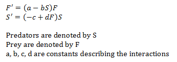
Planar systems are just linear systems in the 2nd dimension. We would like to know how to solve the following systems:

So recall back to the last section, where we discussed eigenvalues λ and eigenvectors v with the solution y(t) = e^λtv. We know that eigenvalues are solutions of the determinant of of A – λI set equal to zero. Let’s expand that out:

This is a quadratic answer, called the characteristic polynomial. Something to note is that the constant term is the determinant of A (without the eigenvalue). For sake of space, we’ll denote this as D (it probably stands for determinant). Then there’s the coefficient of λ, which we’ll denote as T. If you’re in linear algebra, you’ll notice this is the trace of A (or, in other words, the sum of the diagonal entries of A). The trace of A can also be denoted as tr(A). This means we can rewrite our equation of this planar system as

There are three cases we must consider about this characteristic polynomial:

1. Real roots (when T² – 4D > 0)

2. Complex roots (when T² – 4D < 0)

3. A real root of “multiplicity 2” (when T² – 4D = 0)

Here’s a proposition for you:

“Suppose λ₁ and λ₂ are eigenvalues of an n × n matrix A. Suppose v₁ ≠ 0 is an eigenvector for λ₁ and v₂ ≠ 0 is an eigenvector for λ₂. If λ₁ ≠ λ₂, then v₁ and v₂ are linearly independent” (379).

Something really nice to note from this is that if v₁ and v₂ are linearly independent, then

I wanted to actually write that, but there’s only so much that can be done without the equation editor.

Something nice to note about both of these linearly independent conclusions is that the eigenvalues and eigenvectors don’t have to be real for these propositions to be true. If one or more is complex, then the results are still true. Hooray!

Here’s a theorem for you:

“Suppose that A is a 2 × 2 matrix with real eigenvalues λ₁ ≠ λ₂. Suppose that v₁ and v₂ are eigenvectors associated with the eigenvalues. Then the general solution to the system y’ = Ay is

where C₁ and C₂ are arbitrary constants” (380).

In the case of complex eigenvalues, T² – 4D < 0, which would make the square root full of negative-ness, which was a big no-no taught to us on the first day of square roots. However, we can package that negative-ness with the lovely letter i, so our complex roots can look like

This means we’ll have a complex matrix, which I’ll just leave some websites here if you need a refresher on the subject:

 http://www.sosmath.com/matrix/eigen3/eigen3.html

http://tutorial.math.lamar.edu/Classes/DE/ComplexEigenvalues.aspx

http://www.sosmath.com/matrix/complex/complex.html

http://web.eecs.utk.edu/~dongarra/etemplates/node263.html

Here’s a theorem followed by a proposition for you regarding the topic of complex conjugate eigenvalues:

NOTE: You may or may not wonder why I changed one of the eigenvalues from what the book had originally. This is because the book used an overlined λ (also said as “λ bar”) and this will not show up on the website. So I changed it to a strikethrough, which is basically an overline, but moved down a little bit.

“Suppose that A is a 2 × 2 matrix with complex conjugate eigenvalues λ and [λ]. Suppose that w is an eigenvector associated with λ. Then the general solution to the system y’ = Ay is

where C₁ and C_2­ are arbitrary constants” (383).

And the proposition:

“Suppose A is an n × n matrix with real coefficients, and suppose that z(t) = x(t) + iy(t) is a solution to the system z’ = Az.

(a) The complex conjugate [z] =  x – iy is also a solution to [this system].

(b) The real and imaginary parts x and y are also solutions to [this system]. Furthermore, if z and [z] are linearly independent, so are x and y” (383).

So when we have a complex eigenvalue, it will be of the form λ = α + iβ, and its associated eigenvector will be of the form w = v₁ + iv₂. When we have a 2 × 2 matrix A, the solution of the system y’ = Ay will be of the form

where C₁ and C₂ are arbitrary constants” (384).

So now we’re left with the final case for our eigenvalues – the multiplicity 2 one (which is literally called “the easy case” in the book). If this multiplicity nonsense is the case, our characteristic polynomial will be

In this case, λ₁ is T/2 and it has multiplicity 2. This was about the time when I finally realized that multiplicity means something and I don’t think we ever went over it so here’s a thing for you to understand it (like I now do):

 http://math.stackexchange.com/questions/324427/how-to-find-the-multiplicity-of-eigenvalues

From this there are two subcases, depending on the dimension of the eigenspace of λ. Since the eigenspace is a subspace of R², the dimension can only be 1 or 2.

If the dimension is 2, then the eigenspace must be equal to all of R². This means every vector is an eigenvector, so Av = λ₁v for all v in R². For example, if we had

Here’s a theorem concerning the other subcase, where the eigenvalue has λ of multiplicity 2 and eigenspace of dimension 1.

“Suppose that A is a 2 × 2 matrix with one eigenvalue λ of multiplicity 2, and suppose that the eigenspace of λ has dimension 1. Let v₁ be a nonzero eigenvector, and choose v₂ such that (A – λI)v₂ = v₁. Then

form a fundamental set of solutions to the system x’ = Ax” (388).

This means the general solution can be written as

Finally, here's one more website concerning this material that I didn't quite know where to put in this summary: 

http://tutorial.math.lamar.edu/Classes/DE/RepeatedEigenvalues.aspx

All right, that’s it for section 9.2! It wasn’t as bad as I thought it was going to be.

I’ve been ill for the past couple of days, so I’m really foggy right now. I feel pretty good about all this, but if something is blatantly wrong and I don’t pick up on it for a while, then I’m really sorry about that.

I’ll see you when I see you.

9.1, or the extension of chapter 8 (plus eigens)

Chapter 9 is entitled “Linear Systems with Constant Coefficients.”

Section 9.1 is entitled “Overview of the Technique.”

Suppose we’re looking for solutions to the system y’ = Ay. A is a matrix with constant entries (it’s as if they planned for this in the chapter title or something). Let’s start with looking at a first-order and homogeneous equation, which would have the form y’ = ay. The solution for this equation is simple (compared to other examples we could have picked). Since it’s separable, the solution would be y(t) = Ce^at, where C is any constant (which we get from the integration and solving for y(t) and stuff).

So it’s pretty reasonable to look for solution to our system y’ = Ay that have exponentials involved. Let’s look for the solutions that have the form y(t) = e^λtv, where v is a vector with constants for entries (much like A) and λ is a constant we have yet to solve for. If we were to substitute this equation into our original system y’ = Ay, we would get

The exponential factor will never be equation to zero, so we can put these two sides of our equation to together, but only if Av = λv.

As is with most unnamed entities that come from seemingly nowhere in mathematics, v and λ have special names and actually have mathematical roots and are helpful.

 “Suppose A is an n × n matrix. A number λ is called an eigenvalue of A if there is a nonzero vector v such that Av = λv. If λ is an eigenvalue, then any vector v satisfying [this equation] is called an eigenvector associated with the eigenvalue λ” (373).

Something to note about this is that any multiple of v will work as well as an eigenvector.

A big thing to take away from all this is that if λ is the eigenvalue of A and v is the eigenvector, then x(t) = e^λtv is a solution to x’ = Ax. It will also satisfy the initial condition x(0) = v.

Now, your next question might be, “How do we find these eigenvalues?”

So we have this equation Av = λv, which we can rewrite as 0 = Av – λv = Av – λIv = [A – λI]v. Just to remind you, I is the identity matrix. This allows us to factor the v out of the equation, since λ is a mere number and A is a mighty matrix and thus it doesn’t make much sense to write A – λ.

So, in conclusion (and with fancy equation text):

Since v is nonzero (because this is how we defined it), then the matrix A – λI has a nontrivial nullspace. Recall that back in section 7.7 that our pressing issue was how to know whether or not a nullspace was nontrivial. We determined that it’s nontrivial if the determinant was equal to zero, i.e.

So because of the way things turned out, λ will turn up on the diagonals and nowhere else (since the identity matrix is merely ones on the main diagonal, i.e., on the n diagonal terms).  So when we take the determinant, we’ll get a polynomial of degree n in terms of our unknown λ.

“If A is an n × n matrix, the polynomial

is called the characteristic polynomial of A, and the equation

is called the characteristic equation” (374).

This means that eigenvalues of the matrix A are the roots of its characteristic polynomial. We have three choices for roots: real ones, complex ones, and repeated ones.

As if you weren’t already overwhelmed by the amount of eigens floating around, here’s another one for you:

“Let A be an n × n matrix, and let λ be an eigenvalue of A. The set of all eigenvectors associated with λ is equal to the nullspace of A – λI. Hence, the eigenspace of λ is a subspace of Rⁿ” (375).

All right, that’s all 9.1 has to offer you. I guarantee you the next section summary won’t be up until at the very least Friday. My test is on Thursday, and I don’t want these eigens messing up my jive with this test. Thus I will put them to rest for now. I’m approximately two weeks ahead of the weekly schedule, so I’m feeling pretty good at where I’m at with everything (at least enough to be on hiatus for four to five days).

Also, something else to note is that the schedule goes out of order a bit with chapter 9. Just in terms of chapter 9, it goes 9.1, 9.2 + 9.5, 9.6, 9.3, 9.4, 9.7, 9.9, 9.8 + chapter 4, so I might just follow that pattern. Section 9.2 is fairly long (in the sense that I’m not excited to summarize it) so depending on how long summarizing that takes, I might just go in order.

I’ll see you when I see you.

4 chapters down (technically), 3 chapters to go. (8.5)

Section 8.5 is entitled “Properties of Linear Systems.”

I have a feeling a lot of this section will be direct quotes from the book, considering that this section contains quite a few proofs.

“Suppose x₁ and x_2­ are solutions to the homogeneous linear system x’ = Ax. If C₁ and C₂ are any constants, then x = C₁x₁ + C₂x₂ is also a solution to [this system]” (362).

Using the properties of matrix multiplication, we can prove this:

Note that this theorem works if and only if the system is linear and homogeneous.

“Suppose that x₁, x₂, … , and x_k are all solutions to the homogeneous linear system x’ = Ax. Then any linear combination of x₁, x₂, … , and x_k is also a solution. Thus for any constants C₁, C₂, … , C_k, the function

is a solution to x’ = Ax” (363).

So if we have a system, and we want x to be a solution to that system such that x can be expressed as

In this case, x₁ and x_2­ are solutions to our system, and C₁ and C₂ are arbitrary constants. Our goal would be to find C₁ and C₂ which would make our expression of x satisfied for all t. If we know something about our solutions x₁ and x₂, like what their values would be at a specific time/point t, we could solve for C₁ and C₂ at that time/point. We have a handy exactness/uniqueness theorem we can use that would imply our equation would be satisfied for all t. Hooray!

However, something to note that we can only solve our constants provided the matrix

is nonsingular. The matrix will be nonsingular if x₁(t₀) and x₂(t₀) are linearly independent. In this case x­₁₁ and x₁₂ are the values for x₁ at our specific value of t, and x₂₁ and x₂₂ are the values for x₂ at our specific value of t. I suppose I could have made this a little more general, and expanded the rows to contain values x_1n and x_2n, but you get the idea. This works (just in case you’re a little foggy on matrix multiplication) because x(t₀) can be compacted to

The dimension of the first matrix is n × 2, and the dimension of the second matrix is 2 × 1. The multiplication is valid. Double hooray!

Let’s look at a proposition concerning this.

“Suppose y₁(t), y₂(t), … , and (t), … , and y_k(t) are solutions to the n-dimensional system y’ = Ay defined on the interval I = (α, β).

1. If the vectors y₁(t₀), y₂(t₀), … , and y_k(t₀) are linearly dependent for some t₀ ∈ I, then there are contestants C₁, C₂, … , and C_k, not all zero, such that C₁y₁(t) + C₂y₂(t) + … + C_ky_k(t) = 0 for all t ∈ I. In particular, y₁(t), y₂(t), … , and y_k(t) are linearly dependent for all t ∈ I.

2. If for some t₀ ∈ I the vectors y₁(t₀), y₂(t₀), .. , and y_k(t₀) are linearly independent, then y₁(t), y₂(t), … , and y_k(t) are linearly independent for all t ∈ I” (365).

The definition that arises from this is fairly straightforward. If there is one value of t that makes the linear system y’ = Ay linearly independent, then the set of all k solutions of the system is also linearly independent.

“Suppose y₁, …, and y_n are linearly independent solutions to the n-dimensional linear system y’(t) = Ay(t). Then any solution y can be expressed as a linear combination of y₁, …, and y_n. That is, there are constants C₁, …, and C­_n such that

for all t” (365).

If our homogeneous and linear system has a set of n linearly independent solutions, it’ll be called the fundamental set of solutions.

Our last theorem provides us with a way of finding general solutions to the homogeneous system y’ = Ay:

1. Find n linearly independent solutions y₁, y₂, …, y_n.

2. Show the n solutions are linearly independent.

3. Make the general solution

C₁, C₂, …, and C_n are arbitrary constants.

Elaborating on step 2, we only have to show linear independence for one value of t. A great way to do this is to use determinants and the Wronskian. I barely covered this in section 4.1 (which turned out to not be a thing in this class for a while). Hooray! My inability to follow the weekly schedule early on has finally paid off!

If for one value of t, the Wronskian is not equal to zero, then the n solutions are linearly independent.

That’s all for chapter 8! I know I’ll have the time, but if I have the motivation, then I’ll get started on chapter 9.

I’ll see you when I see you.

The section that's combining stuff we've learned from many a chapter - 8.4

Section 8.4 is entitled “Linear Systems.”

Let’s start with what the book means by linear systems. Kind of like linear equations (and by “kind of like” I mean “exactly like”), if there are no products, powers, or higher-order functions, then the functions in a system will appear linearly. This means that a system where the functions appear linearly will be called a linear system.

For example, the following systems are linear:

The following systems are not linear:

Putting things into a more general form, a linear system will have the form

The functions x₁ through x_n are considered to be unknown functions. Known functions are the coefficients a_ij(t) and f_i(t), and are strictly functions of the independent variable. They are defined for all t in a region I = (a, b), which would be an interval in R.

This form is said to be in standard form. Something to note is that there are n unknown functions and n equations; this would make the system’s dimension n. If f_i(t) is zero (for all f_i), then the system is homogeneous. If the f_i(t)s are nonzero, then the system is inhomogeneous.  Thus the f_i(t)s will be called the inhomogeneous parts, or the forcing term. (It’s called a forcing term since, in applications, it arises from external forces.)

The matrix notation for linear systems is as follows:

We can compact all this information in the equation x’(t) = A(t)x(t) + f(t), or x’ = Ax + f.

The three applications of linear systems that are presented in the book are springs (more than one, since this is a linear system), electrical circuits, and mixing problems.

Since this is a summary and all, I could leave it at that, but since I’m a physics major, I’m going to show you electrical circuits. Also, I have a test in this class next week (if you’ve been keeping up, I have a test in differential equations as well. Next week is not going to be a bucket of fun) and the practice could come in handy.

Before I jump on that train of fun times, here are some websites detailing the other two examples.

Springs: http://en.wikipedia.org/wiki/Spring_system and http://www.sosmath.com/diffeq/system/linear/basicdef/basicdef.html

Mixing problems (examples): http://stevesweeney.pbworks.com/f/MPM2D+-+Linear+Systems+07+-+Mixture+Problems+-+W2011.pdf and http://www.purplemath.com/modules/mixture.htm

Here’s a handy recreation of a circuit from the book:

First we use Kirchhoff’s current law to get that I = I₁ + I₂. These are labeled on the diagram by the blue arrows and the I (1) and I (2). 

Kirchhoff’s voltage law tells us that

This is for the loop that contains the voltage source, the resistor, and the inductor. I also reminded you of the physics. (Sometimes I feel like I'm obligated. Sometimes I just don't care if you want physics shoved down your throat or not.) Anyway, when we continue on with our analysis,

For the loop that contains the voltage source, the resistor, and the capacitor, Kirchhoff’s Law tells us

This forms an inhomogeneous and linear system

Finally, to write this system in matrix notation, we’ll have

This system can also be written as I’ = AI + F.

All right, that’s it for section 8.4. I had to write up the last part of this section twice because Microsoft Word is an absolutely perfect and flawless program that will always save my documents in the way I want them to be saved.

I hope to get 8.5 up by tomorrow or Sunday. I also hope to get a review blog post/some sort of note/cheat sheet type of blog post up here too. We’ll see what happens on that, though.

I’ll see you when I see you. 

8.3, a lot of math words about math...words...

Section 8.3 is entitled “Qualitative Analysis.”

Spoiler alert: Solving a system of equations exactly is a rare occasion indeed. Therefore, we’ll need tools to analyze our systems, as to not leave them alone in a corner, allowing them to rot and decay.

As it turns out, we’ll probably be looking at a lot of qualitative analysis in the future. I mean, the systems we can solve are merely a handful of examples of an ocean full of systems of unsolvable equations. The sooner we start, the sooner we finish, right?

Right. Probably. Maybe. I don’t actually know, but let’s just get on with it.

Okay, so what we’re going to be talking about for this section mirrors what we’ve been talking about in previous sections. Perhaps you remember section 2.7, where we talked about exactness and uniqueness. Or perhaps you remember the section we discussed equilibrium points and solutions (I believe it was section 2.9, but I don’t have that section number memorized; remembering 2.9 was pure dumb luck).

Let’s just jump right into the theorems, shall we?

“Suppose the function f(t, x) is defined and continuous in the region R and that the first partial derivatives of f are also continuous in R. Then given any point (t₀, x₀) ∈ R, the initial value problem

has a unique solution defined in an interval contained t₀. Furthermore, the solution will be defined at least until the solution curve t → (t, x(t)) leaves the region R” (348).

This nicely puts exactness and uniqueness into one theorem for us, as to save paper (and our time). Also, you should notice that one of the only differences between this theorem and the theorems for exactness and uniqueness back in 2.7 is that the functions are vector valued.

An important geometric fact that arises from this theorem is that two solution curves in a phase space for an autonomous system (i.e. x’ = f(x)) cannot meet at a point until the curves coincide. However, this does not apply to non-autonomous systems, so just remember what you’re talking about and when.

Here’s a theorem regarding exactness and uniqueness for linear systems:

“Suppose hat A = A(t) is an n × n matrix and f(t) is a column vector and that the components of both are continuous functions of t in an interval (α, β). Then, for any t₀ ∈ (α, β), and for any y₀ ∈ Rⁿ, the inhomogeneous system

with the initial condition

has a unique solution defined for all t ∈ (α, β)” (349).

If the coefficients are constants, then the domain of the system is the entire real line. This means solutions to linear systems with constant coefficients exist on all R.

Now, let’s move onto equilibrium solutions and points.

Let’s look back at our Lotka-Volterra predator-prey model (if you haven’t read 8.2, then I encourage you to stop reading right about now and go read my summary. You could also just Google it and find some webpage. I don’t really mind what you do).

Recall that to find equilibrium solutions, we set our right-hand side equal to zero and solve. For the first equation, you would get F = 0 or A = a/b. In the phase plane, the solution set would be the union of these two lines. This would be called the F-nullcline. Thus, the solution set to the second equation would be the union of S = 0 and F = c/d. This solution set would be called the S-nullcline.

An equilibrium point is where both of these equations are equal to zero. These are the points that are in the intersection of the two nullclines. Therefore, there are two equilibrium points: (0, 0)^T and (c/d, a/b)^T. The equilibrium solutions are

Arbitrarily for an autonomous system x’ = f(x), there will be a vector x₀ which f(x₀) = 0, which will be called an equilibrium point. The function x(t) = x₀ will be called an equilibrium solution.

Here are some websites also summarizing stuff like this: http://www.sosmath.com/diffeq/system/qualitative/qualitative.html

http://mcb.berkeley.edu/courses/mcb137/exercises/Nullclines.pdf

I encourage you to look at nullclines. They’re actually pretty cool. For now, I’ll leave you with 8.3, and 8.4 will be up sometime in the future.

Also, I may or may not write up a pre-test section about important things that will be on my test (supposedly stuff up until and including 7.5). This might be a thing, but it might not. In any event, just know that I probably won’t be summarizing any sections next week. I have to study and prepare, rather than get ahead.

I’ll see you when I see you.

8.2: A lot of words about pretty pictures of graphs

Section 8.2 is entitled “Geometric Representation of Solutions.”

The model we’re going to use this section is called the Lotka-Volterra model of predator-prey populations. I’m not going to derive it; rather, I’ll hand you the final system and you can take my word that it’s all correct:

This model is nonlinear and autonomous.

One way you can represent this model is to plot all of the components of the solution. You can probably Google it (or go here http://en.wikipedia.org/wiki/Lotka%E2%80%93Volterra_equation or here http://mathworld.wolfram.com/Lotka-VolterraEquations.html) but the graphs seem to be a periodic variation of the populations of predators and prey.

Another way we can see the solution is to look at a parametric plot. Let’s set u(t) = (F(t), S(t))^T and plot t → u(t) = (F(t), S(t))^T. This view would be in R², so we can call this solution curve a phase plane.

To see the phase plane of the Lotka-Volterra model, you can go here: http://mathinsight.org/applet/lotka_volterra_phase_plane_versus_time_population_display

For those of you who are too lazy to click on the link (or copy-paste), it looks like an egg. More specifically, it shows how the two populations interact. A fancy term for “egg” is “closed curve”, which means it tracks over itself as time increases. This makes sense, if we are to believe that the solution is indeed periodic. The derivative u’(t) is a vector tangent to our egg at a point u₀ = u(t₀).

This kind of analysis can be done for higher dimensions, (t → y(t) is the parameterization for a curve in Rⁿ, and y’(t) is a vector tangent to the curve at y(t)). It’s just much harder to visualize once you go into dimensions higher than 3.

Now let’s suppose we have a planar system:

In this case, y(t) = (y₁(t), y₂(t))^T would be a solution. We could look at the solution curve t → y(t) in the plane. In this case, this y₁y₂ plane is still called the phase plane, but solution curve is called the phase plane plot or solution curve in the phase plane.

Generally, we’ll be in dimension n and our equation will have the form x’ = f(t, x). The x-coordinates would be called the phase space, and the plot of the curve t → x(t) is called the phase space plot. They’re pretty important for autonomous systems.

Let’s consider the autonomous system

Note this is autonomous because the independent variable doesn’t appear explicitly on the right-hand side. Let’s assume that f and g are defined in a rectangle R in the xy-plane. Let’s consider the solution of the form (x(t), y(t)) and the curve t → (x(t), y(t)) in the xy-plane. This means there will be a vector

that will be tangent to this curve. So if we assign a vector to each point in our rectangle R, then we would have what is called a vector field of our original system. For a pretty picture of the Lotka-Volterra vector field, you can go here http://mathforum.org/mathimages/index.php/Field:Dynamic_Systems#Maps

If we picked a starting point, then the vector field would show us how that curve would form and what our egg would look like. Ultimately, the curve goes back to our original point, which makes sense since we have an egg and not a bowl (or some equivalent open-ended egg shape).

Now let’s start with the general system

Now f and g are defined in a three dimensional shoebox R. This would be in the (t, x, y) space. The limits on this space, in a more general form, would be

In this case, the vector field would be (f(t, x, y), g(t, x, y)), which means it now depends on t, x, and y. Well, if t can change as well, then it doesn’t make much sense to observe a vector field in the phase plane. In this case, we will be looking at a three dimensional direction field.

We’re going to consider the curve parameterized by t → (t, x(t), y(t)) in our shoebox R. This time, our tangent vectors will take the form

Something interesting to note about this is that the vector (1, f(t, x, y), g(t, x, y)) can be computed without knowing the solution of the system. This type of interpretation of our system will be called (surprise, surprise) a direction field.

The solution to the Lotka-Volterra model in a three-dimensional direction field looks really awesome. While my skim of the internet didn’t produce a website that could accurately depict this phenomenon, I encourage you all who have a copy of the book to take a look (page 344).

Since we discussed three different ways to visualize solutions, you can put them all together in a composite graph.

There’s no best way to visualize one of these solutions. The book encourages you to look at all of the visualizations. I encourage you to get correct answers and pass tests (and understand how to visualize these things).

Finally, a thing from the book concerning higher dimensions: “What do we do in higher dimensions? What we do not do is become daunted by the seeming impossibility of visualizing in dimensions greater than 3. Instead we try anything that that seems like it will be helpful” (345).

Don’t be daunted, my friends. I’ll see you when I see you.

Let's talk about diseases: 8.1

Chapter 8 is entitled “An Introduction to Systems.”

Section 8.1 is entitled “Definitions and Examples.”

I’m going to make the observation here and now that any [chapter].1 section will be entirely dedicated to exposition for the succeeding sections.

In other words, [chapter].1 summaries will be particularly dull. I try my best (considering the people who pretend to read/care/enjoy this blog are not emotionally attached to the blog or the class whatsoever, besides my teacher, of course) but for the most part, I don’t have a lot of math jokes/puns to throw at you. Instead, I have math numbers and math words.

Anyway, ready for chapter 8? And the five sections the weekly schedule says we’re covering?

Let’s start off this summary with talking about sick people.

Let’s say there’s a population of people, N. There’s also there’s this disease that’s going around. We have three assumptions about this disease:

1. The disease lasts a short amount of time and doesn’t kill people (not often, anyway).

2. The disease spreads through physical contact.

3. After someone recovers from the disease, he/she will be immune.

Knowing these things, we can split our population N into three groups: people who have never had the disease, people who currently have the disease, and people who have recovered from the disease. We’ll call the first group the susceptible, S(t); the second group will be called the infected, I(t); the third group will be called the recovered, R(t). This means N = S + I + R.

Our first assumption means we can ignore births and deaths. This is nice because N is then constant. Let’s also think about how S(t) will change; susceptible people will catch the disease from infected people and then change groups. This means the rate of change for these two groups is proportional to the number of contacts made. The number of contacts will then be proportional to the product SI of the two populations. This will take the form

In this case, a is a positive constant.

Thinking about how I(t) will change, we think about two different ways. Susceptible people get sick, and infected people get better. We figured out the “susceptible people get sick” part, with our product above. With the “infected people get better part,” this means there will be a rate of recoveries (with some positive constant b). Thus the form will be

Thinking about how R(t) will change, infected people will get better. Thus we already have the form for the rate of change of R:

If we want to wrap everything up in a nice bow, we’ll have

This is called the SIR model. Notice it is nonlinear and autonomous.

The last equation isn’t really needed. The first two equations form a planar and autonomous system. We’ll get the system

This is also referred to as the SIR model.

Notice the SIR model only involves first-order derivatives of the system. It is called a first-order system. Thus we can conclude the order of a system is determined by the highest order derivative in that system. Generally, a first-order system of two equations will have the form

In this case, f and g are functions. A solution to this system would have the form

As always, this will be on some interval of t.

The number of equations should always be equal to the number of unknowns. This will be called the dimension of the system. Thus the system above has dimension 2, and a general system of n equations with n unknowns will have dimension n. A dimension 2 system will be called a planar system.

Notice that our first form of the SIR model is dimension 3, but the second form is a planar system.

If we have a general system

We can write this system in terms of vectors. We can set

One last thing for this section: “…there is a system of first-order equations that is equivalent to any system of higher-order equations, in the sense that a solution to one leads easily to a solution to the other” (335). This means that any application that involves higher-order equations will have an equivalent model with a first-order system. This is nice for the book because we can spend a lot more time studying first-order equations. This is also nice because numerical solvers (remember the two sections from chapter 6?) are more geared toward first-order equations.

Here’s an example of how you can find the first-order system of an equation:

Let’s rename the variables:

So if x solves our original equation, this means that our sets of u functions will solve our new system.

All right, that’s it for section 8.1! Section 8.2 seems a little more yucky than this one, but I’m sure we’ll get by just fine.

I’ll see you when I see you.